www.elsevier.nl / locate / econbase
Environmental regulation and labor demand: evidence
from the South Coast Air Basin
a,b a ,*
Eli Berman , Linda T.M. Bui
a
Department of Economics, Boston University, 270 Bay State Road, Boston, MA 02215, USA b
National Bureau of Economic Research, 1050 Massachusetts Ave., Cambridge, MA 02138-5398, USA
Received 1 February 1999; received in revised form 1 October 1999; accepted 2 October 1999
Abstract
The devolved nature of environmental regulation generates rich regulatory variation across regions, industries and time. We exploit this variation, using direct measures of regulation and plant data, to estimate employment effects of sharply increased air quality regulation in Los Angeles. Regulations were accompanied by large reductions in NOx
emissions and induced large abatement investments for refineries. Nevertheless, we find no
evidence that local air quality regulation substantially reduced employment, even when
allowing for induced plant exit and dissuaded plant entry. Regulations affected employment only slightly — partly because regulated plants are in capital and not labor-intensive industries. These findings are robust to the choice of comparison regions. 2001 Elsevier Science B.V. All rights reserved.
Keywords: Environmental regulations; Employment; Air quality; Effects
JEL classification: J0; J4; L5; L6
1. Introduction
1
The increasing cost of environmental regulation in the past 25 years has fueled
*Corresponding author. Tel.:11-617-353-4140 /11-617-353-6324; fax:11-617-353-4449. E-mail addresses: [email protected] (E. Berman), [email protected] (L.T.M. Bui).
1
American manufacturing plants invested $4.3B in 1994 to abate air pollution (4% of capital investment) and incurred another $6.1B in air pollution abatement operating costs (United States Bureau of Census, 1996). The EPA estimates the cost of abatement for the US at 2.1% of GDP for 1990 (Jaffe et al., 1995).
a debate over its cost-effectiveness in improving environmental quality, and the tightening of national ambient air quality standards in 1997 has intensified that debate. Chief among the perceived costs of regulation is the loss of employment,
2
an issue that looms large in policy debates on environmental regulation. Fears of an inter-regional ‘race to the bottom’ in setting lax environmental regulations to avoid local job loss was one reason for the establishment of the US Environmental Protection Agency (EPA). In light of such concerns, efficient (and politically feasible) regulation requires precise estimates of its effects on employment.
Environmental regulation does not necessarily reduce labor demand. While abatement activities probably increase marginal costs and decrease labor demand through reductions in sales, abatement activities may, in fact, complement labor — leading to an increase in labor demand. Theory alone yields an ambiguous prediction of the over-all employment effects of environmental regulation. Existing empirical studies have likewise yielded mixed results on these
employ-3
ment effects (Jaffe et al., 1995).
Estimating the effects of environmental regulation is difficult for a number of reasons. Some studies have estimated the effects of regulation by regressing outcomes on measured abatement activity (see for example, Gray and Shadbegian (1993b). This approach is confounded by selection bias and measurement error. Plants that can abate at low cost are likely to have the smallest employment effects and are most likely to abate voluntarily — without the impetus of regulation. This selection effect will bias estimates of the effects of induced abatement on employment, making abatement appear less costly than it actually is. Measurement error in abatement costs also is likely to bias estimated effects toward zero because of attenuation bias.
Our solution to these estimation problems is to gather detailed micro data on local air pollution regulations in a specific region of the country and to construct relevant treatment and comparison groups for each industry affected by the local air quality regulations that we study. Comparison groups are constructed to represent the counterfactual in which treated plants are not subject to local air pollution regulation. We code regulations as binary indicators and estimate the
2
For example, in California, employment effects must be taken into account in the formulation of environmental regulations (Sept. 1994, resolution 94-36, South Coast Air Quality Management District).
3
effect of regulation on employment directly (rather than the effect of abatement expenditures on employment).
The richness of our data comes from the structure of US environmental regulation. Since the EPA delegates much regulatory authority to state and local agencies, regulatory stringency varies across regions for the same industries, depending upon local environmental quality. We focus on the manufacturing sector in this paper. Our innovation is in directly estimating the effects of local air pollution regulations using a quantitative approach that includes comparison plants in the same precisely defined industry. This allows us to check the robustness of our results by alternating the regions used for comparison plants. To implement this approach we quantify local air pollution regulations as binary covariates, a lengthy procedure that involves numerous subjective judgements. Our principal methodological contribution is a coding procedure that avoids bias due to ‘data mining’ using a simple method we call ‘sequestering the data.’
The Los Angeles area provides our study with an episode of sharp increase in local air quality regulation in the 1980s. These local regulations apply over and
above federal and state regulations. The South Coast Air Quality Management
District (SCAQMD), which regulates the air basin containing Los Angeles and her
4
suburbs, has enacted some of the country’s most stringent air quality regulations since 1979. These were triggered by the interaction of increasingly stringent air quality standards and abysmal air quality in the South Coast. Poor air quality is due both to emissions and topographical conditions: the unique climate and geography of the region contribute to a thermal inversion, which traps pollutants near ground level. Thus the SCAQMD found itself far out of compliance with the 1970 EPA national ambient air quality standards. It responded by the late 1970s, adopting a set of extremely stringent regulations in an attempt to meet those standards, an effort primarily aimed at reducing emissions of nitrous oxides (NO ).x
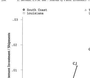
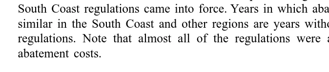
For example, Fig. 1 illustrates the costs imposed by these regulations on South Coast oil refineries, the most highly regulated of manufacturing industries. Beginning in 1986, when these regulations came into effect, South Coast refineries faced much higher abatement investment costs than did refineries in Texas and Louisiana, regions with less stringent state regulations and no local air quality
5
regulation. The strict and sometimes innovative approach to environmental regulation in the South Coast has been copied by other regions in their attempts to comply with the national ambient air quality standards. The increased stringency of 1997 EPA air quality standards may eventually force adoption of similar regulations in other regions, so estimated employment effects of South Coast regulations should be of interest to regulators elsewhere in the country.
4
The South Coast Air Basin consists of Los Angeles County, Orange County, Riverside County, and the non-desert portion of San Bernardino County.
5
Fig. 1. Abatement investment / value of shipments in refineries. Source: PACE survey. Notes: The graph compares air pollution abatement investment in oil refineries in the South Coast region to that in the refineries of Texas, Louisiana and the entire US. Abatement investment is calculated from the PACE survey. Each compliance date for a South Coast regulation is labeled with a ‘C’ and each date of increased stringency is labeled with an ‘I’. For instance, in 1991 one regulation had a compliance date and two had dates of increased stringency. Abatement investment data are unavailable in 1983 and 1987.
regulations. Our estimates are of the effect of local South Coast regulations in contrast to the average level of local regulation in the comparison regions. We report separate estimates using attainment and non-attainment comparison regions, as well as a Texas–Louisiana comparison region, which has a similar industrial structure to the South Coast but less stringent air pollution regulation.
To match the degree of detail in regulatory variation we use two panels of plant level data made available to us by special arrangement with the Census Bureau: the Pollution Abatement Costs and Expenditures Survey (PACE) in 1979–1991 and the Census of Manufactures in 1977, 1982, 1987 and 1992. These data allow us to identify plants subject to new South Coast regulations and to compare them with plants (plant-years to be precise) not subject to new regulations. Using this approach we can remove potentially confounding plant effects, and industry and / or region specific shifts in employment in estimating the effect of regulatory change on employment. In an analysis of the Los Angeles area during the 1980s these are key issues, as the regional concentration of declining defense industries led to a secular decline in employment which we argue has been falsely attributed to environmental regulation. We claim that the incidence of regulation is orthogonal to sample selection because the timing of regulation was due to the confluence of the stringency of federal (EPA) air quality standards and the serious air quality problem in Los Angeles.
We find that while regulations do impose large costs they have a limited effect on employment. Compliance with a new regulation induces $0.5M of abatement investment per affected plant (with a standard error of $0.2M). Increases in stringency of an existing regulation induce $1.9M ($1M) of abatement investment. The employment effects of both compliance and increased stringency are fairly precisely estimated zeros, even when exit and dissuaded entry effects are included. Point estimates of the cumulative effect of 12 years of air quality regulation from 1979–1991 vary according to the comparison regions used, from 2600 to 5400 jobs created, with standard errors about the size of the estimates. Point estimates based on the quintennial Census (which allow for entry and exit of plants, long term response and include 1992 regulations as well) vary more with comparison groups, from 9600 jobs lost to 12 300 jobs gained. These are very small effects in a region with 14 million residents and about 1 million manufacturing jobs. The large negative employment effects alluded to in the public debate (Goodstein, 1996) can clearly be ruled out.
Small employment effects are probably due to the combination of three factors: (a) regulations apply disproportionately to capital-intensive plants with relatively little employment; (b) these plants sell to local markets where competitors are subject to the same regulations, so that regulations do not decrease sales very much; and (c) abatement inputs complement employment.
activity an indicator for whether a county attains compliance with federal standards. They both find that transition into attainment is associated with an incursion of polluting plants. Greenstone also finds negative employment, invest-ment and output effects for continuing plants. Gray (1997) finds that states with more stringent enforcement have fewer plant openings. Levinson (1996) examines plants in pollution intensive industries, finding little impact of regulation on the location of new manufacturing plants (1982–1987).
This paper is related in method to a recent literature in labor economics and public finance that uses cross-sectional variation in changes in regulations, laws and institutions to study the effects of these changes. The variation is often arguably exogenous and the results are of interest to policy makers contemplating similar regulatory changes. Meyer (1995) provides a survey. We offer two innovations to that literature: first, we demonstrate that useful regulatory variation can come from a set of diverse, technical regulations once they are appropriately quantified. Second, we show that geographical variation observed within industry in plant data allows the use of comparison plants in different regions to test the robustness of the estimates.
Several characteristics of local air quality regulation programs make our approach an attractive alternative to existing evaluation methods. Air quality regulation is too expensive to allow random assignment of treatment. Similar to the job training programs discussed by Hotz et al. (1998), local air quality regulation efforts involve a mixture of components applied to a population with distinct characteristics. In these situations Hotz et al. (1998) stress the need for precise measurement of the characteristics of program components and of the treated population to allow prediction of a program’s effects on other populations. It is hard to imagine an approach not based on micro regulations and plant level data that satisfies the two critical conditions for credible estimation: (a) enough detailed information on industry and regional characteristics to remain uncon-founded by secular trends, and (b) enough comparison regions so that there is sufficient overlap in characteristics between treatment and comparison groups to allow estimation.
The paper proceeds as follows. Section 2 provides background about en-vironmental regulation in the SCAQMD. In Section 3, we derive estimating equations from a model of labor demand under regulation. Section 4 describes the data. In Section 5, we present results and Section 6 concludes.
2. Background: the regulation of air quality
The national standards are based on health criteria alone, not on economic cost-benefit analyses. For air pollution, these national ambient air quality standards (NAAQS) apply to six ‘criteria’ air pollutants (sulfurous oxides, nitrous oxides, particulate matter, volatile organic compounds, ozone, and airborne lead). States are responsible for state implementation plans (SIPs) which the EPA must approve. The plan indicates how the state will ensure that all its regions attain the standards. The EPA can withhold federal funds from states without approved SIPs and has threatened to take over environmental regulation in California if the state does not comply with the NAAQS.
Federal environmental regulation of stationary sources is generally limited to new sources of pollution (New Source Performance Standards, ‘NSPS’), except in ‘non-attainment’ regions that do not meet the federal standards and in regions deemed ‘pristine’ (Prevention of Significant Deterioration regions, or ‘PSD’). In non-attainment regions all new investment must meet the ‘lowest achievable emissions rate’ standard. In pristine regions new investment must meet the less severe ‘best available control technology’ standard. Both the ‘lowest achievable’ and ‘best available’ standards are more demanding than the NSPS. New sources of pollution and major modifications to existing sources are restricted in both regions. All other sources of pollution, including existing stationary sources and mobile sources generally are regulated at the state level.
In California, air pollution from mobile sources is regulated by the California Air Resource Board, while the regulation of stationary sources is delegated to 34 local air quality management districts. The South Coast Air Quality Management District (SCAQMD) is responsible for the South Coast Air Basin in the area
6
around Los Angeles. The South Coast is further from attainment of the NAAQS than any other large region, hence the unprecedented severity of regulations which came into force in the mid-1980s.
Severe air pollution in the Basin is partly due to weather patterns. The Basin is arid, with little wind, abundant sunshine, and poor natural ventilation — conditions that exacerbate air pollution, especially the formation of ground level
7
ozone. It is densely populated with high concentrations of motor vehicles and industry. In 1990, the Basin contained 4% of the US population and 47% of the population of California.
When the NAAQS were first established, the Basin was out of attainment for four of the six criteria pollutants. Hall et al. (1989) report that non-attainment of federal standards between 1984 and 1986 increased the death rate by one in ten
8
thousand (a risk that doubles in San Bernardino and Riverside Counties). Over
6
In 1977, Orange, Riverside, and the non desert portion of San Bernardino Counties joined the Los Angeles County Air Pollution Board to form the SCAQMD.
7
Ozone is produced by a combination of volatile organic compounds, NO and sunlight.x
8
half the Basin’s population experienced a stage 1 ozone alert annually, during which children were not allowed to play outdoors. The average resident suffered 16 days of minor eye irritations and 1 day on which normal activities were substantially restricted.
The South Coast responded with local air quality regulations, over and above those imposed by the EPA and the State. These included heavy regulation of industrial emissions, generally mandating emission reductions and investment in emission control equipment. Table 1 illustrates the associated increase in abate-ment costs. Between 1979 and 1991 South Coast manufacturing plants increased air pollution abatement costs by 138%, nearly twice the national rate of increase, and increased air pollution abatement investment by 127%, ten times the national rate of increase. South Coast oil refineries incurred the lion’s share of increased abatement costs, accounting for the majority of abatement investment and
9
operating costs by 1991.
Fig. 1 illustrates the effect of these regulations on abatement investment in oil refineries, where most measured abatement took place. The top line reports abatement investment as a proportion of shipments in South Coast refineries, while the other three report that proportion in the refineries of Texas, Louisiana and the entire US. Refinery abatement investment is much higher than that in the comparison regions in 1986, 1988, 1990, 1991 and 1992. The letters ‘C’ and ‘I’ indicate a South Coast refinery regulation with a compliance or an increased stringency date in that year, respectively. All years with a large gap between South Coast abatement and abatement in the comparison regions are years in which South Coast regulations came into force. Years in which abatement investment is similar in the South Coast and other regions are years without new South Coast regulations. Note that almost all of the regulations were associated with high abatement costs.
Table 1
a Air pollution abatement control expenditures (Millions of 1991 Dollars)
Capital Expenditures Operating Cost South Coast US South Coast US
1979 101 3313 125 2820
1991 229 3703 298 4978
% Growth
1979–91 127 12 138 77
a
Source: Authors’ calculations from PACE micro data. Figures are slightly smaller than published totals for US Manufacturing.
9
Regulation significantly improved ambient air quality. Between 1976 and 1993 the Basin reduced out-of-attainment days by 47%, from 279 to 147. The South Coast program emphasized decreasing NO emissions (primarily to reduce ozone,x
but also to reduce PM10 and because the federal NO standard was attainable). Fig.x
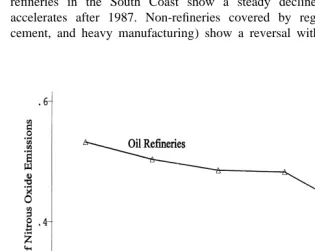
2 illustrates the role of local, as opposed to state or federal, regulation in reducing NO emissions by manufacturing plants. It shows the share of South Coast plantsx
in California’s NO emissions in three categories of manufacturing: oil refineries;x
other plants affected by local regulations in the South Coast; and plants not affected by South Coast regulations. The comparison to plants in the same industries in the rest of California allows a contrast with the effects of state and federal regulations over and above which the South Coast regulations apply. Oil refineries in the South Coast show a steady decline in NOx share, which accelerates after 1987. Non-refineries covered by regulations (e.g. chemical, cement, and heavy manufacturing) show a reversal with an increasing share of
Fig. 2. Relative decline in South Coast NO emissions by regulatory category. Note: The figurex
10
state emissions after 1985. Plants not covered by South Coast regulations reduced emissions no faster than did comparable plants in the rest of California. Despite this regulatory effort, in 1993 the South Coast remained out of compliance for three other criteria air pollutants (PM , ozone and CO) and still had the10
highest annual average NO level in the nation.x
3. Labor demand under environmental regulation
In this section we motivate our estimating equations with a model of labor demand that allows regulation to act through two separate mechanisms, the output elasticity of labor demand and the marginal rates of technical substitution between abatement activity and labor. The partial static equilibrium model of production (Brown and Christensen, 1981) allows for the levels of some ‘quasi-fixed’ factors to be fixed by exogenous constraints, rather than by cost minimization alone. We apply that approach, treating costs incurred to comply with environmental regulation — pollution abatement capital investment and abatement costs (labor, materials and services) — as ‘quasi-fixed’. Labor, materials and productive (regular) capital are the variable factors.
Assume a cost-minimizing firm operating in perfectly competitive markets for inputs and output. There are J variable inputs and K ‘quasi-fixed’ inputs. The variable cost function has the form:
CV5H(Y, P , . . . , P , Z , . . . , Z )1 J 1 K (1) where Y is output, the P are prices of variable inputs, and Z are quantities ofj k
quasi-fixed inputs. Profit maximization implies the first order conditions that yields demand for the variable input labor, L, as a function of output, quantities of the
11
other inputs, and prices, which we approximate by the linear equation:
K J
L5a 1 rYY1
O
bkZk1O
gjP .j (2)k51 j51 10
In the period between 1983–85 and 1990–91 NO emissions declined by 15 000 tons (standardx
error56600) in South Coast refineries and by 5400 tons (7300) in other California refineries. NOx
emissions declined by 8300 tons (4200) in other regulated South Coast plants but increased by 11 900 tons (13 300) in plants in the same industries in the rest of California. Standard errors are calculated using raw data on point sources, corrected for heteroskedasticity, grouped plant effects and industry effects.
11
The reduced form effect of regulation (R) on labor demand can be written:
L5d 1 mR. (3)
The effects of regulation on employment are through the mechanism:
K J
dP dZ
dL dY k j
]dR5rY]dR1
O
bk]dR1O
gj]dR5m. (4)k51 j51
If input markets are large and competitive, regulatory change will have no effect on input prices so the final term in (4) will disappear, leaving the first two. The first term reflects the effect of regulation on demand for variable factors through its effect on output. This output effect of environmental regulation is widely believed to be negative (though theory gives no clear prediction: if compliance is achieved through an investment that reduces marginal costs, dY / dR could be positive). The second term reflects the effect of regulation on demand for variable factors through its effect on demand for quasi-fixed abatement activities, Z, and the marginal rates of technical substitution between abatement and variable factors. The change in demand for abatement activity due to an increase in regulation, dZ / dR, must be positive.
The signs of the bk, which reflect whether abatement activity and labor are complements or substitutes, are not known a priori. Abatement technologies fall into two general categories, ‘end-of-pipe’ and ‘changes in process.’ End-of-pipe technologies such as scrubbers and precipitators, remove pollutants from existing discharge streams before their release into the environment, and probably complement labor, particularly production labor. Improvements in production process, such as the installation of more efficient boilers which operate at lower levels of emissions, often reduce demand for production workers due to a general skill-bias of technological change. Hence the signs of thebk are ambiguous, which is the main reason that the sign ofm, the employment effect of regulation, cannot
12
be predicted from theory alone.
Some of the employment effects of regulation may be through induced exit of plants, as output is reduced to zero, and through dissuaded entry (Henderson, 1996; Levinson, 1996; Gray, 1997). For those effects only the output effect (the
12
first term of (4)) is relevant, so the employment effect of regulation through induced exit and dissuaded entry is likely to be negative.
4. Data description
We exploit variation in regulation across industries, regions and time by using plant level data. We use two (unbalanced) panels drawn from Census Bureau data: The Survey of Pollution Abatement and Control Expenditures (PACE), linked to the Annual Survey of Manufactures (ASM), and the Census of Manufactures (CM). (Plant records from the ASM linked over time are the basis of the Longitudinal Research Database (LRD) panel compiled by the Center for Economic Studies of the Census Bureau).
The ASM samples the population of manufacturing plants, including large plants (250 or more employees) with certainty. Smaller plants are rotated out of the sample at 5-year intervals. From these data we use the employment, value added, and capital investment variables. PACE reports abatement investment and operating costs by the medium abated (air, water, and hazardous waste). We use air pollution abatement costs and investments. To account for entry and exit we use the Census of Manufactures, which covers the population of manufacturing plants
13
every 5 years. From these data we make use of employment, value added, and capital investment. These data are described fully in an appendix available from the authors.
Our most difficult task was the construction of measures of regulatory change. We constructed a data set for the Basin detailing all changes in local environmen-tal regulation affecting manufacturing plants from 1979–92. We identified 46 separate local air regulations, many affecting multiple industries, and tracked their adoption and compliance dates as well as dates of increased stringency. We used local regulatory code books, the SCAQMD library, interviews with regulators and regulatees to establish the timing and coverage of regulations. Regulations were matched to industries using the text of the regulation, our understanding of
14
production technologies, and information provided by South Coast regulators. Manufacturing plants located in Texas and Louisiana are our primary com-parison group because the composition of industry in those states is similar to that
13
A plant is a physical location engaged in a specific line of business. Plants with 20 or more employees are required to submit a survey form to the Census, while smaller plants are often enumerated using payroll and sales information from the Social Security Administration and the Internal Revenue Service. Imputed plants account for approximately 2.2% of value added (United States Bureau of the Census, 1993).
14
15
in the South Coast, but air pollution regulations are less stringent. For alternate comparison regions we used ozone attainment / non-attainment regions according
16,17
to their 1987 status.
Coding regulations carries with it an inherent danger of bias. Regulations have enough technical attributes that coding involves numerous subjective judgements. For instance, a regulation requiring capital investment with compliance early in the year will force a plant to invest during the previous year, so it is coded as occurring in the previous year. If the researcher carrying out the coding has even a vague idea of the pattern to be explained, then subjective judgement implies a danger of (inadvertently) ‘data mining’, by coding the data in a way that will help explain variation in the left hand side variable (in our case, employment). Our solution for is to ‘sequester’ the data, not allowing the researcher who codes the regulations to observe the left hand side variables. We believe that this method of sequestering the data is crucial to obtain unbiased inferences from micro-regula-tory data, especially in a case like ours in which the collection and coding of regulations is an expensive activity which does not lend itself to corroboration by replication.
We developed an exhaustive coding of significant South Coast regulations for the 1979–92 period. To achieve precision we interviewed regulators and a sample of regulatees both personally and by telephone. Regulations are concentrated in heavy industry (paper, chemicals, petrochemicals, glass, cement, and transport). Regulatory data were matched to each of the two panels of plants (ASM-PACE and COM). For each plant-year we measure the number of new regulations adopted, new regulations that must be complied with and the number of
15
In discussions with several individuals, we found that this opinion was widely held by regulators in the South Coast as well as plant engineers in companies with plants in both the South Coast and either Texas or Louisiana. When a direct comparison was possible between regulations in the South Coast and those in Texas and Louisiana, South Coast regulations were clearly more stringent B between two and ten times more stringent on a per unit emissions standard basis. For example the SCAQMD ([1159) requires that NO emissions from nitric acid units be no more than 3 pounds per ton of acid per 60 min2 whereas in Louisiana the limit is 6.5 pounds per ton. At present, there are no other specific regulations for nitrous oxide emissions in Louisiana other than those for nitric acid units. Gas fired steam generators in the South Coast ([1146, 1146.1) are limited to between 30 and 40 ppm per MMBTUs of heat input (0.037–0.04 lbs per MMBTUs of heat input) but in Texas (in the Dallas / Fort Worth ACQR and Houston / Galveston ACQR) the limit is 0.25–0.7 lbs / MMBTUs. The cost of the South Coast regulation on gas fired steam generators is estimated at between $9161 and $16 635 per ton in 1990$, or $3.9–$4.6M per year.
16
Another measure of regulatory stringency is effort expended by the regulators, including enforcement activities, as proxied by budgets. The SCAQMD’s budget is, on average, eight times as large as that of the Louisiana Air Quality Program and in 1999 was approximately the same size as that of all of Texas for their Clean Air Account. Thus the South Coast spends approximately 2.5 times as much per capita on air pollution control as Louisiana and 1.3 times as much as Texas.
17
regulations with increases in stringency. For example, Rule 1112 applies an emission standard to NO emissions from cement kilns. The Rule was adopted in2
1982 and had a date of compliance in 1986. These regulatory data are available from the authors upon request.
For comparison plants we include in each panel all US manufacturing plants located outside of the Basin in industries that would have been affected by SCAQMD regulations had they been located there.
5. Estimation
5.1. Econometrics
We are interested in estimating the effect of the South Coast regulations on employment in regulated plants. We first describe the estimating equation and then discuss how we deal with potential sources of bias.
The effect of regulation on labor demand, given by Eq. (3), can be taken to data as:
Lijrt5d 1 f 1 mi t Rjrt1h 1 v 1 ejt rt ijrt. (39)
The unit of observation is a plant-year. The parameterm is the effect of regulation on employment;diis a plant-specific employment effect for i51, . . . , N plants;t ft
is a year effect for years t51, . . . , T; hjt is an industry effect for industries
j51, . . . , J; and vrt is a region effect for regions r51..R. We eliminate the plant-specific effect by differencing to yield:
DLijrt5 Df 1 mDt Rjrt1 Dh 1 Dv 1 Dej r ijrt (5)
assuming employment trends Dh and Dv in industries and regions respectively. The parameter of interest, m, can be consistently estimated if Cov(DR ,De )5
jrt ijrt
0.
The assumed orthogonality of regulatory change with unexplained variation in employment change is conditional on year, industry and region indicators. This conditioning is critical. Regulatory change is certainly bunched in particular years, which typically have their own secular employment change. Particular industries and regions also have their own secular patterns of employment change. The orthogonality assumption is a claim that regulatory changes are correlated with employment changes only through the causal effectm, once the common effects of time, industry and region are taken into account.
(more stringent) SCAQMD regulations over and above the average level of regulation (Federal and State) these industries face in the rest of the country. Since the level of regulation varies from region to region, the estimated effects should be interpreted as an average of separate cross-region comparisons.
Before turning to results, we discuss three potential sources of bias we believe apply to this literature and explain how our identification strategy deals with them.
5.1.1. Selection bias
This is the first effort we know of to estimate the effects of local air quality regulations directly in an analysis including comparison plants. An alternative approach which indirectly measures these effects is to estimate (2) directly, using abatement activity (Z ) as a covariate in a labor demand function. That approach avoids the considerable effort described above of quantifying regulations but is susceptible to selection bias. Plants may carry out PACE voluntarily even in the absence of regulation, a phenomenon that is probably more common at plants that anticipate small disruptions due to PACE (Gray, 1987). Such a selection bias would tend to yield estimates which understate negative employment effects of PACE forced by regulation, which is the relevant parameter for policy analysis. Selection bias may explain the surprising Gray and Shadbegian (1993b) result that PACE is positively correlated with employment.
5.1.2. Measurement error
PACE is difficult to measure for two reasons. First, the distinction between investments in pollution abatement capital and other new capital is often subtle (Jaffe et al., 1995). For example, new equipment is frequently both more efficient and cleaner. Second, the survey form defines PACE as the difference between capital investment and the counterfactual capital investment that would be made in the absence of the need to abate. While this is exactly the definition an analyst would like, it is a difficult question for a respondent to answer. After years of air quality regulation that counterfactual may be difficult to imagine, as it is far removed from experience. This is a type of measurement error, which, in the regression of employment on abatement, will generally bias coefficient estimates towards zero.
5.1.3. Anticipatory response
managers, who indicated that anticipatory abatement investment is unlikely, as compliance typically involves high costs which they would not incur until it was absolutely necessary. We estimate (5) in both annual and 5-year differences to capture both short term and long term responses.
We describe regulations using three binary indicators, one for the year of required compliance, a second for the year in which an existing regulation became
18
more stringent and a third for the date of adoption of the regulation. For each indicator the coefficient estimates the average treatment effect, averaged over all South Coast regulations introduced during this period.
5.2. Result from a balanced panel
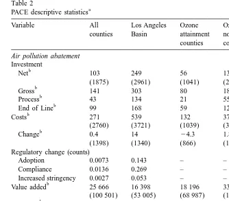
Our ASM-PACE panel contains 18 540 plant-years in industries that would be subject to South Coast regulations if they were located in the LA air basin. They represent 60 500 plants in the population. The panel contains data for 1979–1991, excluding 1983 and 1987 (for which data were destroyed and not collected, respectively). Table 2 reports means and standard deviations, weighted by sampling weights to reflect population statistics. The means indicate that in these industries abatement investment and operating costs are high, averaging $103 000 and $271 000 per plant, respectively. Abatement costs vary considerably among plants, with standard deviations an order of magnitude larger than the means. This reflects the large costs incurred by a small number of petrochemical and chemical plants. Note that 5.3% of plant-years are located in the LA Basin. The compliance indicator averages 1.36%. The average year to year change in employment is210, which reflects the national contraction in manufacturing employment in heavy industry over the 1980s. In comparison with plants in the same industries in other regions, South Coast plants are smaller and have higher proportions of abatement
19
investment and operating cost to value added.
We begin by presenting the estimated effects of regulation on employment from Eq. (5), using changes in regulation to explain year to year changes in employ-ment. Regulatory changes, DR , take values of zero, one and sometimes two forjrt
South Coast plants and are always zero for plants in other regions. The vector
DRjrt includes new regulations adopted (but which require no immediate action), new compliance dates and dates of increased stringency of existing regulations. While we expect the effects of regulation to occur in compliance years and years of increased stringency, the adoption year indicator is included to allow for
18
Strictly speaking these are counts, since more than one new regulation sometimes applies to a plant in a given year, so that DR, while generally binary, can take values of up to 4 over the 5-year differences reported for the CM below. Coefficients should be interpreted as the average effect of a single regulation.
19
Table 2
a PACE descriptive statistics
Variable All Los Angeles Ozone Ozone Texas–
counties Basin attainment nonattainment Louisiana
Gross 141 303 80 184 316
b
Process 43 134 21 55 116
b
End of Line 99 168 59 129 200
b
Costs 271 539 132 379 896
(2760) (3721) (1039) (3677) (6664)
Compliance 0.0136 0.269 – – –
Increased stringency 0.0027 0.053 – – –
b
Employment 267 178 205 323 212
(867) (350) (585) (998) (533)
Change 210 26 25 215 26
(173) (117) (98) (221) (106)
LA Air Basin (%) 5.3 100 – – –
Observations 18 540 964 6973 9483 2086
a
Notes: Means weighted by LRD-PACE sampling weights. In all, 18 540 sample observations represent 60 500 plant-years in the population of manufacturing plants over the sample period 1979–1991, excepting 1983 and 1987 when data is unavailable. Standard deviations in parentheses. Attainment indicates that the county is below the federal ozone guideline for ambient air quality in 1987. All plants in the LA air basin are in nonattainment counties. Attainment / nonattainment classification is not available for a small number of counties.
b
Thousands of 1991 dollars deflated by PPI.
possible anticipatory response. Note that regulations vary widely in their spe-cifications and potential effects so that estimated effects should be interpreted as average treatment effects.
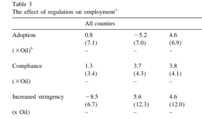
Table 3 reports estimated coefficients. Employment effects are very small,
20
generally positive, but not statistically different from zero. The first three
20
Table 3
a The effect of regulation on employment
All counties
Increased stringency 28.5 5.6 4.6 2.9
(6.7) (12.3) (12.0) (15.8)
(x Oil) – – – 7.2
(17.1)
36 industry indicators – 1 1 1
50 state indicators – – 1 1
N 18 540 18 540 18 540 18 540
2
R 0.011 0.023 0.026 0.026
c
Program effect 2292 3948 3862 4100
(2938) (3590) (3487) (3413) a
The dependent variable is plant-level employment, first-differenced. Weighted by PACE-LRD sampling weights. Each estimate includes 9-year indicators and an indicator for the South Coast Air Quality Management District. Standard errors in parentheses are heteroskedasticity consistent. The mean employment change is210.
b
‘3Oil’ is in each instance a variable set to one if a regulatory change (e.g. adoption) occurred and it affected the petroleum industry (SIC code 2911).
c
Program effects are the sum of affected plants multiplied by estimated coefficients for compliance, increased stringency and their interactions with oil, where applicable.
columns indicate that these small estimated coefficients are robust to controlling for industry and state effects. The specification allowing industry and state specific year to year employment changes yields point estimates of an additional 3.8 employees in compliance years and an increase of 4.6 employees in years of increased stringency (which occur about one fifth as often). These estimates do not rule out zero or negative effects of regulation on employment, but they do rule out the large negative effects (‘job loss’) often attributed to environmental regulation in the popular press. There is no evidence that adoption dates matter, a point to which we return, below. As so much abatement cost is incurred by refineries, we report separate effects for refineries and non-refineries, which are also all small.
stringency date with an ‘I’. Only regulations applying outside refineries (SIC 29) are marked as refinery employment is relatively small and shows little variation over this period. Ten of 16 compliance and increased stringency dates occur in 1990–91, so it is not surprising that environmental regulations were fingered as the cause of the employment decline.
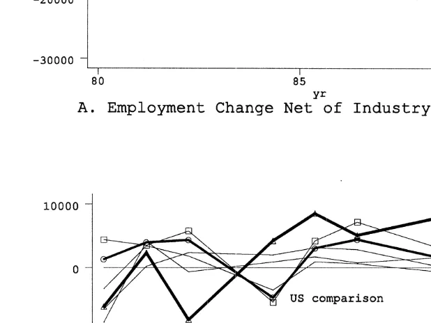
The second series illuminates how the estimates in Table 3 exonerate air quality regulations. We constructed that series by first regressing changes in employment on year and industry indicators, as in column 2 of Table 3, excluding regulation variables. We then summed the employment change residuals for the South Coast, creating an employment change series net of national period effects and national industry-specific employment trends. That series shows no decrease in employ-ment in 1990 or 1991, indicating that the heavy job loss experienced in the South Coast in those years is due to a high proportion of declining industries. Once national industry-employment trends are netted out, there is little job loss left for local regulations to explain.
The coefficients on compliance and increased stringency dates can be used to estimate the cumulative effect of the set of 1980–1991 environmental regulations of manufacturing plants in the South Coast, reported in the last row as the ‘program effect.’ The point estimate using the specification in the rightmost column is a 4100 person increase in employment with a 95% confidence interval ranging from 3570 jobs lost to 11 770 jobs gained. Using the lower bound of that confidence interval as a worst case, job loss due to regulation was probably less than 3570 — a small number, having the same order of magnitude as the estimated
annual rate of excess deaths from being out of compliance with national standards
in the mid 1980s.
Interpretation of these coefficients as the causal effects of regulation depends critically on the assumption that, in the absence of regulation, the treated plants would have behaved like the comparison plants, conditional on industry, region and year. Industry indicators are good predictors of the propensity of comparison plants to be treated (i.e. subject to South Coast regulations) had they been located
21
in the South Coast, since industries share production technologies across regions and since the incidence of regulations is based either on process or directly on industry.
A possible weakness of our approach is that a small number of our comparison plants may be subject to some degree of region-specific environmental regulation
22
that is promulgated at the state level. Thus, the treatment effects estimated must be interpreted as the effects of the difference between South Coast regulations and the average level of a small number of location-specific state regulations in comparison regions. We address this issue in two ways. First, since
location-21
In interviews, production engineers indicated that they used largely the same capital goods as competing firms and as plants in the same firm in other regions.
22
specific state regulations are triggered by non-compliance with federal air quality standards, we compare (the treated) South Coast plants with plants in both attainment and non-attainment regions for federal ozone standards in 1987. Since we expect that non-attainment regions have more stringent local regulations, on average, the contrast between their outcomes and those of the South Coast plants is particularly interesting. These are also the regions for which the results are most relevant, as they are most likely to adopt the more stringent South Coast regulations.
Our second approach is to draw comparison plants from Texas and Louisiana, which have a pollution intensive industrial mix, with large petroleum refining and heavy industry sectors. Unlike the South Coast, these two states benefit from topological and climactic conditions that make them much less prone to accumu-late ground level ozone. We directly compared state regulations in these two states with the local regulations in the South Coast and found that they were much less stringent (see footnotes 15 and 16).
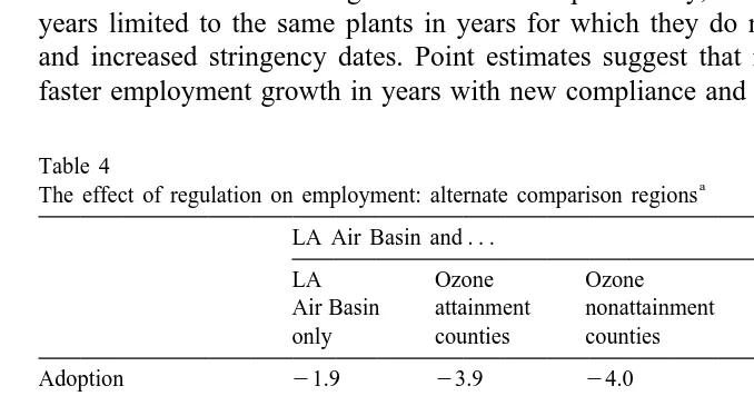
Table 4 describes the outcome of both approaches. The leftmost column reports estimated coefficients using the South Coast plants only, with comparison plant-years limited to the same plants in plant-years for which they do not have compliance and increased stringency dates. Point estimates suggest that regulated plants had faster employment growth in years with new compliance and increased stringency
Table 4
a The effect of regulation on employment: alternate comparison regions
LA Air Basin and . . .
LA Ozone Ozone Texas– All
Air Basin attainment nonattainment Louisiana counties only counties counties
Adoption 21.9 23.9 24.0 0.5 4.6
(9.6) (6.8) (7.4) (7.0) (6.9)
Compliance 5.8 3.9 3.9 3.4 3.8
(4.6) (3.6) (4.9) (4.1) (4.1)
Increased stringency 9.0 23.5 13.8 21.2 4.6
(16.4) (8.6) (15.2) (12.5) (12.0)
36 industry indicators 1 1 1 1 1
50 state indicators – 1 1 – 1
N 964 7937 10 447 3050 18 540
2
R 0.050 0.023 0.033 0.022 0.026
b
Program effect 6219 2643 5424 2652 3862
(3870) (3188) (4094) (3673) (3487)
a
Dependent variable is plant-level employment, first-differenced. Weighted by PACE-LRD sampling weights. Each estimate includes 9-year indicators and an indicator for the South Coast Air Quality Management District. Standard errors in parentheses are heteroskedasticity consistent. The mean employment change is 210.
b
dates than in other years, (thought the effect is not statistically significant). The other columns report estimates which contrast employment growth for South Coast plants with employment change in plants in the same industries in comparison regions. That contrast generally reduces the estimated employment effects slightly, but does not make them significantly negative in any case. Estimated program effects are all positive, with lower bounds on their confidence intervals predicting small employment losses at worst. The conclusion from comparisons with plants in attainment counties, non-attainment counties and the relatively unregulated States of Texas and Louisiana is always the same: employment effects are fairly
precisely estimated and small. This robustness to the choice of comparison groups
is illustrated in panel B of Fig. 3, which plots employment change as in panel A and net employment change using each of the five comparison groups in Table 4. All five comparisons yield the same conclusion: secular industry effects alone can explain the rapid decline in South Coast employment in 1990 and 1991. This is true even when these trends are estimated using as a comparison region ozone attainment counties that were subject to neither South Coast nor other local regulations.
Considering these small and statistically insignificant employment effects a legitimate question is whether environmental regulation did anything economically significant in manufacturing plants. In terms of Eq. (4), was there a ‘first stage’ effect of regulation on abatement and output? Fig. 2 provided one response, showing that regulations induced reduced emissions. It reported sizeable NOx
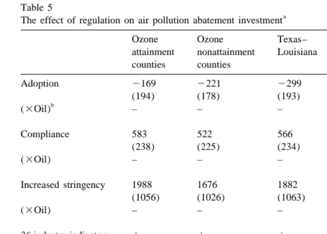
emissions reductions in regulated South Coast plants after 1985, in both refineries and non-refineries, much faster than the reductions in unregulated South Coast plants. Table 5 provides another response, showing the result of estimating the analogous equation to (5) for abatement investment. It is estimated in first differences with year to year changes in abatement capital (net abatement investment) on the left hand side and DR on the right. The results show that
compliance and increases in regulatory stringency have large and significant effects on abatement investment. The units are thousands of dollars (constant 1991$) so that the coefficient on compliance in the leftmost column implies $583 000 of capital investment induced by each new regulation per affected plant. The estimated effect of increased stringency is larger, but somewhat less precisely estimated. The point estimates in column 1 indicates that increased stringency induces an additional $2M in investment per plant. These results are robust to changes in comparison regions. Those coefficients clearly indicate that the South Coast regulations imposed large costs on manufacturing plants.
The first row indicates no evidence that adoption of regulations has any effect on abatement investment. The evidence is weak, but consistent with the opinion of environmental engineers we interviewed, who reported that anticipatory invest-ment was unlikely because the high cost of abateinvest-ment investinvest-ment.
Table 5
a The effect of regulation on air pollution abatement investment
Ozone Ozone Texas– All All
Compliance 583 522 566 553 217
(238) (225) (234) (234) (39)
(3Oil) – – – – 2730
(1052)
Increased stringency 1988 1676 1882 1807 2256
(1056) (1026) (1063) (1044) (147)
(3Oil) – – – – 7016
(2937)
36 industry indicators 1 1 1 1 1
50 state indicators 1 1 – 1 1
N 7937 10 447 3050 18 540 18 540
2
R 0.057 0.057 0.073 0.041 0.058
c
F-statistic 4.61 3.96 4.10 4.24 4.77
(a) (0.01) (0.02) (0.02) (0.01) (0.001)
d
Program effect 802 907 701 842 771 881 748 772 415 164 (265 037) (251 221) (271 544) (258 065) (120 721) a
Dependent variable is plant-level pollution abatement capital investment (air), first-differenced. Weighted by PACE-LRD sampling weights. Each estimate includes 9-year indicators and an indicator for the South Coast district. Standard errors in parentheses are heteroskedasticity consistent. The mean of net air pollution abatement investment is 103 (1000s of 1991$s).
b
‘3Oil’ is in each instance a variable set to one if a regulatory change (e.g. adoption) occurred and it affected the petroleum industry (SIC code 2911).
c
The F-statistic reports the results of an F-test of the hypothesis that the coefficients on compliance and increased stringency are jointly equal to zero. The number in parentheses is the significance level at which that hypothesis can be rejected.
d
Program effects are the sum of affected plants multiplied by estimated coefficients for compliance, increased stringency and their interactions with oil, where applicable.
estimates in Table 5 are a first stage. Those reduced form estimates would be subject to the same biases we seek to avoid in OLS estimates if the first stage had only a weak correlation between regulatory change and investment (Bound et al., 1995). For that reason we report near the bottom of Table 5 an F-test of the joint hypothesis that the coefficients on both compliance and increased stringency are zero. The F-statistics are all around four, indicating negligible bias in the reduced form (Bound et al., 1995, Table A1).
effects for other industries insignificantly different from zero. These contrast with the results in Fig. 2, which find NO reductions in both refineries and in otherx
regulated industries.
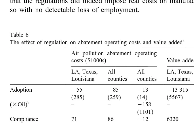
Table 6 repeats that procedure for abatement operating costs and value added respectively. We find no evidence that regulatory change has any effect on abatement operating costs or value added. The data may be uninformative because differencing the levels of abatement cost and value added exacerbates measure-ment error. Measuremeasure-ment of abatemeasure-ment operating costs is especially suspect because its variation from year to year seems to be unreasonably high.
Taken together, the results in Tables 3–5, and Fig. 2 provide an interesting contrast. Though air quality regulation induced large investments in abatement capital in oil refineries, and NO reductions in general, what little effect it had onx
employment seems positive, if anything. The evidence of a ‘first stage’ effect of regulations on abatement, together with evidence of reduced emissions, indicates that the regulations did indeed impose real costs on manufacturing firms, but did so with no detectable loss of employment.
Table 6
a The effect of regulation on abatement operating costs and value added
Air pollution abatement operating
costs ($1000s) Value added ($1000s) LA, Texas, All All LA, Texas, All All Louisiana counties counties Louisiana counties counties
Adoption 255 285 213 213 315 211 958 2533
(285) (259) (14) (5567) (5178) (1639)
b
(3Oil) – – 2158 – – 246 123
(1101) (19 811)
Compliance 71 86 212 6320 5748 486
(126) (113) (10) (3419) (3210) (963)
(3Oil) – – 688 – – 16 737
(451) (16 027)
Increased stringency 2500 2508 215 214 2992 21955 (452) (416) (19) (10 238) (8983) (1663)
(3Oil) – – 22168 – – 1094
R 0.003 0.001 0.002 0.012 0.010 0.011
a
Dependent variable is plant-level pollution abatement operating and maintenance costs (air), first-differenced. Weighted by PACE-LRD sampling weights. Each estimate includes 9-year indicators and an indicator for the South Coast Air Quality Management District. Standard errors in parentheses are heteroskedasticity consistent. The mean change in air pollution operating costs is 0.4 (1000s of 1991$s) and the mean change in value added is 598 (1000s of 1991$s).
b
5.3. Entry and exit analysis using the census of manufactures
Environmental regulation may influence employment by inducing plants to exit or dissuading them from entering into production. A limitation of the ASM results above is that entry and exit are not recorded in a panel of continuing plants so that
23
potential employment effects of regulation have gone unmeasured. Cost-mini-mizing behavior predicts that employment effects are more likely to be negative through induced exit and dissuaded entry than they are for continuing plants (Eq. (4)), since technical complementarity between abatement and employment requires
24
production. To capture the effects of regulation through exit and dissuaded entry we turn to the quintennial Census of Manufactures, the most complete data on manufacturing employment available from any source. As before, our sub-population includes plants which would have been subject to South Coast regulations had they been located in the South Coast. Comparison regions represent counterfactual patterns of employment change, including entry and exit, which would have occurred in the South Coast in the absence of regulations. Pooling all three types of employment change, we estimate the effects of regulation through forced exit, dissuaded entry and changes in employment in continuing plants.
One weakness of the Census to Census comparison is that over a 5-year period other events may occur in regulated industries in the LA Basin or elsewhere that confound analysis of the effects of regulation. One such event is the sharp decrease in orders for defense-related goods as the federal government reduced spending on ‘Star Wars’ and other programs. This led to considerable job loss in the aerospace industry, which is disproportionately concentrated in Southern California, an industry that was subject to two relatively minor environmental regulations in the 1987–92 period. Most of these industries were affected by one VOC regulation concerning coatings, which had a compliance date of January 1993, long after their sharp downturn in employment. To control for fluctuations in defense procurement we use a sub-population of regulated industries in the CM to exclude the aerospace
25
and shipbuilding industries.
The effect of changes in regulation on changes in employment in Eq. (5) is estimated for departing and entering plants as follows: plants entering are assigned zero employment in the census year before they appear and plants departing are assigned zero employment in the census year after they exit. Employment levels are then used to calculate five year differences for all plants, including continuing
23
The Annual Survey of Manufacturers changes its sample of smaller plants periodically so that entry and exit are not well observed and are practically indistinguishable from plants joining and leaving the sample.
24
Regulation could also induce entry of plants which produce abatement producing equipment. None of the industries covered by the South Coast regulations fall into that category.
25
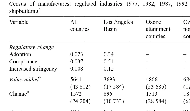
Table 7
Census of manufactures: regulated industries 1977, 1982, 1987, 1992 excluding aerospace and a
shipbuilding
Variable All Los Angeles Ozone Ozone Texas–
counties Basin attainment nonattainment Louisiana counties counties
Regulatory change
Adoption 0.023 0.34 – – –
Compliance 0.037 0.54 – – –
Increased stringency 0.008 0.12 – – –
b
Value added 5641 3693 4866 6846 7252
(43 812) (17 584) (53 685) (124 925) (40 402) b
Change 1572 896 1513 1811 1920
(24 204) (10 733) (28 584) (62 338) (24 189)
Employment 68.6 51.5 65.1 76.6 69.5
(328.2) (148) (397.6) (998) (245.5)
Change 22.1 21.5 1.9 25.3 20.8
(158.6) (81.7) (195.9) (221) (113.4)
LA Air Basin (%) 6.7 100 – – –
Observations 142 613 9604 68 294 77 898 10 933
a
A total of 142 613 observations of 5-year differences, covering the periods 1977–82, 82–87, 87–92. Value added and employment levels are based on observations for the years 1982, 1987 and 1992. The sub-population includes all 46 regulated industries listed in Table A2 with the exception of six aerospace industries and shipbuilding (SIC codes 3721, 3724, 3728, 3761, 3764, 3769 and 3731).
b
Value added is reported in thousands of constant 1991 dollars.
plants. Note that this method also allows an estimate of a longer term response over the 5-year intervals.
Table 7 reports three periods of 5-year changes in employment: 1977–82, 1982–87 and 1987–92. Average employment change for a plant over these 5-year periods was 22.1 employees, including employment increases for entrants and decreases for exits. Regulatory change is added up for the 5-year intervals between Census years. Plants outside the South Coast are assigned no increase in regulations over the 5-year intervals. Plants in the South Coast had between zero and five new compliance dates for regulations. The average for all plants was 0.037 new compliance dates and 0.008 dates of increased stringency.
As in the PACE-LRD sample, comparison regions are chosen with varying levels of state regulation. Table 8 reports estimates of Eq. (5) which allow for exit and entry. The first column reports results including all (non-defense) plants, including entrants and exiting plants. Employment effects per new compliance regulation vary from 12.8 (for the Texas–Louisiana comparison group) to 22.4 (for non-attainment counties). Effects of increased stringency vary from 15.6 to
23.2.
Table 8
Effects of regulation on employment between census years 1977–82, 1982–87, 1987–92: alternative a
comparison regions
LA Air Basin and . . .
Ozone Ozone Texas– All All counties
attainment nonattainment Texas– Louisiana counties (including counties counties Louisiana entry / exit only aerospace)
Adoption 20.5 5.4 22.9 21.8 3.4 6.6
(2.1) (2.2) (2.2) (2.8) (2.0) (6.1)
Compliance 21.1 22.4 2.8 3.1 22.0 28.3
(1.3) (1.4) (1.4) (1.9) (1.3) (4.7)
Increased stringency 23.2 5.6 22.2 23.3 1.6 11.3
(3.7) (3.8) (4.2) (6.0) (3.5) (6.1)
b
Industry indicators 1 1 1 1 1 1
c
State indicators 1 1 1 1 1 1
N 63 154 77 898 20 537 12 107 142 613 151 908
2
R 0.009 0.008 0.009 0.015 0.005 0.003
d
Program effect 29589 26140 12 266 7047 28860 234 286 (8545) (8678) (9632) (8348) (8303) (23 479) a
Heteroskedasticity-consistent standard errors in parentheses. The sample is described in Table 7. Dependent variable is 5-year changes in plant-level employment.
b
All columns include 39 four-digit industry indicators except for the rightmost, which includes an additional seven in aerospace and shipbuilding. These seven industries are subject to a relatively minor VOC regulation with a compliance date in the first quarter of 1993.
c
From the leftmost column, the number of state indicators is respectively 42, 32, 2, 51 and 51 (including Puerto Rico). All columns include a separate indicator of the South Coast.
d
Program effects are the sum of affected plants multiplied by estimated coefficients for compliance and increased stringency.
the Louisiana–Texas comparison group for which we are most confident that there is relatively little local air quality regulation. Surprisingly, we find coefficients of similar size for exitors and entrants on the one hand and for continuing plants on
26
the other. The effects for both entry / exit and continuing plants are small, positive and not statistically distinct from zero. This positive point estimate on compliance is a little surprising for the exit / entry sample (though statistically insignificant) especially since it is larger than that estimated for continuing plants. (This is true
26
for the full sample as well, though not reported.) While it may be due to misclassification of continuing plants as exit / entry combinations, it underlines the finding of no large negative employment effect through induced entry and exit. Other comparisons (not reported) yield similar results.
The final column reports the effect of ignoring the bias due to a procurement drop in the South Coast and including defense-related industries. That estimate would imply large negative employment effects. As discussed in connection with Fig. 3, the confusion between the effects of decreased defense contracts and environmental regulation may be why regulation was falsely implicated in the employment loss in South Coast manufacturing.
Overall, these coefficient estimates are more negative but statistically in-distinguishable from the estimates based on annual employment and regulatory change reported in Tables 3 and 4 above, providing corroboration of those results in a different data set, over a longer time period and including exit and entry effects. The similarity of the annual and quintennial results is evidence that these estimated employment effects are not subject to measurement error bias or confounded by lagged or anticipated response. As in the annual data, neither of these figures is statistically different from zero, but the standard error is small enough to rule out large employment effects, both positive and negative.
The coefficients allow a fairly precise estimate of the cumulative effect on employment of the 1980–92 period of air quality regulation in the South Coast: point estimates range from 9600 jobs lost when compared with attainment counties, to 12 300 jobs created when compared to Louisiana and Texas (excluding the last column which includes aerospace industries). The 95% confidence interval in the worst case is [226 338, 7160] and in the best case is [26613, 31 145], so that at standard levels of confidence we can bound the employment effects of the entire program between about 26 000 jobs lost and
27
31 000 jobs gained.
Comparing the Census estimates of employment effects to those in the annual ASM-PACE samples, the latter are generally more positive. While the Census estimates have the advantage of broader coverage, including entry and exit effects, they are also reported at lower frequency, increasing the probability of a confounding secular industry–region–period event, such as the drop in defense procurements. Finally, they are not completely comparable since they include an extra year of regulation, in 1992. Nevertheless, the Census estimates generally reinforce the conclusion of small employment effects found in the ASM-PACE data in Tables 3 and 4. Air quality regulation in the South Coast did not cause large scale job loss even when dissuaded entry and exit and longer term adjustment are taken into account.
27
6. Conclusion
The local air quality regulations introduced during 1979–92 in the Los Angeles Basin were not responsible for a large decline in employment. In fact, they probably increased labor demand slightly. We reach that conclusion by directly measuring regulations and comparing changes in employment in affected plants to those in comparison plants in the same industries but in regions not subject to South Coast regulations. Our ability to construct appropriate comparison groups in regions without local regulation is the key to identifying treatment effects and to establishing the robustness of these estimates.
Reduced form estimates alone are uninformative about why these employment effects are small. One possible explanation is that the program had no economic effect on the subject plants. That possibility, however, is ruled out by our considerable evidence of induced abatement investment in refineries and of induced abatement of NO emissions in both regulated refineries and regulatedx
non-refineries.
Another possible explanation for small employment effects is that South Coast regulations targeted capital intensive industries with relatively little employment. This is certainly true of oil refineries but also true of chemicals, cement, transportation and other heavy manufacturing. Thus, our conclusions may extend to environmental regulation in other regions only to the extent that they affect capital-intensive industries (which they often do).
Plant visits and phone surveys support another explanation (suggested by theory) that, on the one hand, output effects of regulation may be small, while on the other, that labor and abatement activity are compliments. Most managers we spoke to thought that the introduction of abatement technology increased labor demand. While all complained about the nuisance of dealing with regulators and complying with regulations, few complained about lost demand for their product. We speculate that this is because these plants sell to local markets and face little competition from unregulated plants (in the oil and chemical industries).
Our estimates of zero employment effects contradict the conventional wisdom of employers (mostly outside of refining) that environmental regulation ‘costs jobs’ (Goodstein, 1996) so a comment is in order. Beyond posturing in public debate, employers may honestly overestimate the job loss induced by a pervasive regulation by confusing the firm’s product demand curve with that of the industry. The former is more price elastic due to competition from other firms. If all firms in the industry are faced with the same cost-increasing regulatory change and product demand is inelastic, the output of individual firms may be only slightly reduced. In that case, the negative effect on employment through the output elasticity of labor demand may well be dominated by a positive effect through the marginal rate of technical substitution between PACE and labor, leading to a net increases in employment as a result of regulation.
regulation only do so at the latest possible moment — adoption dates have no discernible effect on a plant’s investment whereas mandatory compliance dates have a strong effect. This is not surprising given the large capital investment associated with coming into compliance with a given regulation.
Though the public debate has centered around employment effects, a full accounting of the costs of regulation should properly focus on the effects of regulation on productivity and the benefits in health and other outcomes. Related research on South Coast refineries (Berman and Bui, 1998) has found productivity gains between 1987–92, in contrast to declining productivity in comparison regions. A symmetric analysis of the benefits of the South Coast regulations in improved air quality and health outcomes of residents would form the basis for a much more complete economic evaluation of this important and unprecedented episode in air quality regulation.
Acknowledgements
This research was supported by the Canadian Employment Research Foundation and National Science Foundation grant SBR95-21890, through the National Bureau of Economic Research. We thank Joyce Cooper of the US Census Bureau Boston Research Data Center and Mary Streitweiser at the Census Bureau Center for Economic Studies for constructing and helping us interpret the database. We appreciate the comments of Jim Poterba and two thoughtful anonymous referees, as well as the comments and assistance of Wayne Gray, Vernon Henderson, Kevin Lang and Theodore S. Sims and the comments of participants in the CERF conference ‘Sustainable Development and the Labor Market,’ Ottawa and semi-nars at Harvard, MIT, UBC, Princeton, McMaster, Boston University, the Hebrew University, Tufts, Tel Aviv University, the California Institute of Technology, the National Bureau of Economic Research and CREST (Paris). We thank Zaur Rzakhanov and Noah Greenhill for research assistance. All remaining errors are our own. The research in this paper was conducted while the authors were Census Bureau research associates at the Boston Data Research Center. Research results and conclusions expressed are those of the authors and do not necessarily indicate concurrence by the Bureau of the Census. The paper has been screened to insure that no confidential data is revealed.
References