A GENERAL CLASS OF NONLINEAR UNIVARIATE SUBDIVISION
ALGORITHMS AND THEIR C2 SMOOTHNESS
Esfandiar Nava-Yazdani
Abstract. Considering subdivision schemes in nonlinear geometries, it is
nat-ural to define an analogues subdivision of a linear one in terms of some functions and new variables reflecting the geometry. In the present work we introduce the notion of analogues of a given linear subdivision in a general setting such that some important examples like log-exponential subdivision in Lie groups (also infinite di-mensional applications) are covered. Moreover, we prove that C2 smoothness of the
linear subdivision implies the same property for the analogues one. Moreover, we present some applications to Lie groups and symmetric spaces.
2000 Mathematics Subject Classification: 41A25, 26B05, 22E05, 68U05
Keywords and phrases: Nonlinear subdivision,C1andC2smoothness, Lie groups,
Log-Exponential scheme
1.Introduction
In view of the wide range of applications of subdivision processes in nonlinear geometries there has been a growing attention to this topic in the recent years. Many important such applications arrise in continum mechanics by consideration of data corresponding to strain or stress tensor, or in elasticity (deformation tensors) as well as medical imaging (diffusion tensors). Further examples are provided by situations when data naturally live in some Lie groups, for instance vehicle headings or motion of rigid body. For a comprehensive study of many important examples we refer to [5].
properties using the general methods introduced in [7] and [6] has been established in [7], [9] and [8]. For further readings on smoothness of subdivision of manifold- or Lie group-valued data we also refer to [10] and [2].
Definition of the mentioned analogue subdivision schemes uses tangent vectors and the Riemannian exponential map or resp. the exponential map of the Lie group. An important task is then, to understand the relation between convergence and smoothness of the linear subdivision and the analogues nonlinear one.
In the present work we introduce the notion of analogues of a given linear sub-division in a general setting such that some important examples like log-exponential subdivision in Lie groups (also infinite dimensional applications) are covered. More-over, we prove that C2 smoothness of the linear subdivision implies the same
prop-erty for the analogues one, provided the linear subdivision scheme and its difference schemes up to order 3 satisfy certain boundedness conditions.
2.Analogues of a subdivision
Let (E,k k) ba a Banach space, N > 1 an integer and a := {ai}i∈Z a finite
sequence in E with
X
j∈Z
al−jN = 1, l= 0, . . . , N −1. (1)
We denote the linear subdivision associated to the sequence a by S, i.e. Spl+iN =
X
j∈Z
al−jNpi+j (2)
for a sequence of pointsp:={pi}i∈Z (control points). The number of rulesN is called
dialtion factor, the sequence a mask and the Laurent polynomial a(z) := P
i∈Zaiz
i
associated to a the symbol of S. Condition (1) ensures convergence of Sp for all p and is called affine invariance.
Suppose that f : M ×E → M is C2 with the following (local) properties: each
x∈M has a neighbourhood U such that
f(x,0) =x, (3)
D1f(x,0) =IdE, D2f(x,0)−1 exist, (4)
D11f(x,0) = 0, D12f(x,0)(D2f(x,0)v, w) =D22f(x,0)(v, w) for all v, w∈E. (5)
Now, suppose that the pointspi are close enough in the following sence. p⊂U ⊂
M such thatf|U enjoys the above properties. For simplicity we denote the restriction
of f toU byf. Then the equations
pi+1 =f(pi, vi) (6)
define a sequence of vectors v :={vi}i∈Z inE. Now we define thef-analogue ofS as
T pl+iN =f(pi,
X
j∈Z
al−jN(vi+j−1+· · ·+vi)), l = 0, . . . , N −1. (7)
Note that (7) can be written as T pl+iN =f(pi,
X
k∈Z
( X
j−1≥k
al−jN)vi+k, l= 0, . . . , N −1. (8)
We also denote that by (3)
f(f(. . .(f(x,0),0), . . . ,0) =x. (9) As all considerations in the present work are local, we may and do assume U ⊂E.
3.Smoothness
In the next two subsections we summarize some notions and facts which will used to prove smoothness. For the corresponding background material we refer to [6]. We denote the forward difference operator ∆ operating on the vector space of sequences in E by ∆, i.e.,
∆i+1p:= ∆(∆ip), ∆0p:=p.
3.1.Derived schemes and proximity
Derived (also called difference) schemes of the subdivision scheme S are defined by
By affine invariance the first derived scheme S1 always exist. Derived schemes up
to order k exist if and only if a(z) is divisible by (1 +z +· · ·+zN−1)k. We denote
µk := N1kSkk.
To prove smoothness properties of the analogue subdivision scheme we use the method of the so-called proximity conditions. We first need the following technical lemmas.
Lemma 1. Suppose that derived schems of S up to order n exist. Denote ckl := (X
j∈Z
jal−jN)k−
X
j∈Z
jkal−jN, l= 0, . . . , N −1. (10)
Then the following holds
∆jcj+1l = 0 for all l = 0, . . . , N −1 and j = 1, . . . , n−1. (11) Proof. Denoting ξ:=e2πi/N, existence of derived schemes up to ordern is equivalent
to
N−1
X
l=0
X
j∈Z
(l+jN)(l−1 +jN). . .(l−n+ 1 +jN)al+jNξk(l−n) = 0
for k = 1, . . . , N −1. These equations can be written as
N−1
X
l=0
X
j∈Z
(l+jN)(l−1 +jN). . .(l−n+ 1 +jN)al+jNξkl = 0.
with k = 1, . . . , N −1. Defining αn,l:=
X
j∈Z
(l+jN)(l−1 +jN). . .(l−n+ 1 +jN)al+jN,
we see that αn,l is independent of l and in view of N−1
X
l=0
αn,l =a(n)(1)
we have αn,l = a
(n) (1)
N . Denoting bn,l :=
P
j∈Zjnal+jN and
Pn
i=0σi,lzi := (l+z)(l−
1 +z). . .(l−n+ 1 +z) it follows that bn,l is given by the recursion formula
bn,l =
1 Nn+1(a
(n)(1)− n−1
X
i=0
Hence bn,l and bn1,l are polynomials inl of degree n with equal coefficients of (n−
1)-th resp. n-th monomial (given by (−N1)n−1na′(1) resp. (−1 N )
n). Therefore ∆ncn+1 l =
(−1)n+1∆n(bn
1,l−bn,l) = 0.
Lemma 2. There are positive constants C and C′ such that
kvk ≤Ck∆pk (12)
k∆vk ≤C′(k∆2pk+k∆pk2) (13) Proof. Since f(pi, .) is a local deiffeomorphism, there is C >0 such that
Ckvik ≤ kf(pi, vi)−f(pi,0)k=kpi+1−pik=k∆pik
holds. This proves the first inequality. Moreover, linearization of ∆2p
i at v = 0 gives
∆2pi =f(f(pi, vi), vi+1)−2f(pi, vi) +pi
=D2f(pi,0)∆vi+o(kvik2).
Using (12) we get the inequality
k∆vik ≤ kD2f(pi,0)−1k(k∆2pik+o(kvk2))kD2f(pi,0)−1k(k∆2pik+Ck∆pk2)
from which (13) immediately follows.
Lemma 3. (i) There is a positive constant C such that
kSp−T pk ≤Ck∆pk2 (14)
(ii) Suppose that S2 and S3 exist. Then there exist a positive constant C′ such that
kSp−T pk ≤C′(k∆pkk∆2pk+k∆pk3) (15)
Proof. A straighforward calculation shows that
∂vkpj =
(
D1f(pj−1, vj−1). . . D1f(pk+1, vk+1)D2f(pk, vk) for k = 0, . . . , j−1.
0 else
Ad i) For l = 0, . . . , N −2 the linearization of ∆Spl+iN at v = 0 reads as
∆(T p−Sp)l+iN (1)
=X
j∈Z
X
k≤j−1
al+1−jND2f(pi,0)vi+k
−X
j∈Z
X
k≤j−1
al−jND2f(pi,0)vi+k
−X
j∈Z
X
k≤j−1
al+1−jN(D1f(pi,0))j−k−1D2f(pi,0)vi+k
+X
j∈Z
X
k≤j−1
al−jN(D1f(pi,0))j−k−1D2f(pi,0)vi+k
For l =N −1 we have ∆(T p−Sp)l+iN
(1)
=D1f(pi,0)D2f(pi,0)vi+
X
j∈Z
X
k≤j−1
a−jND2f(pi,0)vi+1+k
−X
j∈Z
X
k≤j−1
a−1+(1−j)ND2f(pi,0)vi+k
−X
j∈Z
X
k≤j
a−jN(D1f(pi,0))j−kD2f(pi,0)vi+k
+X
j∈Z
X
k≤j−1
a−1+(1−j)N(D1f(pi,0))j−k−1D2f(pi,0)vi+k
Using D1f(pi,0) =Id and affine invariance we arrive at
∆(T p−Sp)(1)= 0 from which the desired inequality follows.
Ad ii) In view of (16) we have ∂vi+k′∂vi+k′pi+j = 0 for k /∈ {0, . . . , j −1} or k
′ ∈/
{0, . . . , j−1}. Furthermore for k, k′ = 0, . . . , j−1 ∂vi+k′∂vi+kpi+j
=∂vi+k′D1f(pi+j−1, vi+j−1)D1f(pi+j−2, vi+j−2). . . D1f(pi+k+1, vi+k+1)D2f(pi+k, vi+k)
+D1f(pi+j−1, vi+j−1)∂vi+k′D1f(pi+j−2, vi+j−2). . . D1f(pi+k+1, vi+k+1)D2f(pi+k, vi+k)
...
+D1f(pi+j−1, vi+j−1). . . ∂vi+k′D1f(pi+k+1, vi+k+1)D2f(pi+k, vi+k)
Therefore we have 2Spl+iN
(2)
=X
j∈Z
al−jN[
X
k≤j−1
(X
k′=k
((j−k−1)D11f(pi,0)(D2f(pi,0)vi+k, D2f(pi,0)vi+k′)
+D22f(pi,0)(vi+k, vi+k′))
+X
k′<k
((j −k−1)D11f(pi,0)(D2f(pi,0)vi+k, D2f(pi,0)vi+k′)
+D12f(pi,0)(D2f(pi,0)vi+k′, vi+k))
+X
k′>k
((j −k′ −1)D11f(pi,0)(D2f(pi,0)vi+k′, D2f(pi,0)vi+k)
+D12f(pi,0)(D2f(pi,0)vi+k, vi+k′))]
Using D11f(pi,0) = 0 and D12f(pi,0)◦D2f(pi,0) =D22f(pi,0) we arrive at
2Spl+iN (2)
=X
j∈Z
al−jN
X
k′,k≤j−1
D22f(pi,0)(vi+k, vi+k′), l = 0, . . . , N −1.
For l =N −1 we may write 2Spl+1+iN = 2
X
j∈Z
a−jNpi+j+1 (2)
=X
j∈Z
a−jN
X
k′,k≤j
D22f(pi,0)(vi+k, vi+k′)
=X
j∈Z
a−jN(
X
k′,k≤j−1
D22f(pi,0)(vi+1+k, vi+1+k′) +
X
k≤j−1
D22f(pi,0)(vi+k+1, vi)
+ X
k′≤j−1
D22f(pi,0)(vi, vi+k′+1) +D22f(pi,0)(vi, vi))
=X
j∈Z
aN−jN
X
k′,k≤j−1
D22f(pi,0)(vi+k, vi+k′) +
X
j∈Z
a−jN(
X
k≤j−1
D22f(pi,0)(vi+k+1, vi)
+ X
k′≤j−1
D22f(pi,0)(vi, vi+k′+1)) +D22f(pi,0)(vi, vi).
Moreover for l = 0, . . . , N −1 2T pl+iN
(2)
= X
k,k′∈Z
and for l =N −1 2T pl+1+iN
(2)
= X
k,k′∈Z
a−kNa−k′ND22f(pi,0)(vi+1+· · ·+vi+k, vi+1+· · ·+vi+k′)
+X
k′∈Z
a−k′ND21f(pi,0)(D2f(pi,0)vi, vi+1+· · ·+vi+k′)
+X
k∈Z
a−kND21f(pi,0)(vi+1+· · ·+vi+k, D2f(pi,0)vi)
+D22f(pi,0)(vi, vi)
= X
k,k′∈Z
aN−kNaN−k′ND22f(pi,0)(vi+· · ·+vi+k−1, vi+· · ·+vi+k′−1)
+X
k′∈Z
a−k′ND22f(pi,0)(vi, vi+1+· · ·+vi+k′)
+X
k∈Z
a−kND22f(pi,0)(vi+1+· · ·+vi+k, vi)
+D22f(pi,0)(vi, vi).
Now denotingck,kl ′ = (P
k≤j−1al+1−jN
P
k′≤j−1al+1−jN−
P
k≤j−1al−jN
P
k′≤j−1al−jN)−
P
k,k′≤j−1(al+1−jN−al−jN) and writing the second order Taylor expansion of ∆(T p−
Sp)l+iN as
∆(Sp−T p)l+iN =P(v) +o(kvk3)
we arrive at
P(v) = X
k,k′∈Z
Ak,k′(vi+k, vi+k′)
where
Ak,k′ =ck,k ′
l D22f(pi,0).
Note that
P(v) = X
k,k′∈Z
Ak,k′(v0, v0) +
X
k,k′∈Z
(
k−1
X
l=0
Ak,k′(∆vl, vj) +
k′−1
X
l=0
In view of Lemma 1 we further have P
k,k′∈ZAk,k′ =
P
k,k′∈Zc
k,k′
l D22f(pi,0) = 0.
Hence we can write
∆(Sp−T p)l+iN =
X
k,k′∈Z
(
k−1
X
l=0
Ak,k′(∆vl, vj) +
k′−1
X
l=0
Ak,k′(v0,∆vl)) +o(kvk3).
Applying the triangle inequality to the above equation and using lemma 2 we imme-diately arrive at the desired estimate.
3.2.Main results
In this section we present our main results as follows. 1If the derived schemes of
the linear subdivision scheme S up to order 3 exist and their norm satisfy certain inequalities, then the analogues nonlinear scheme is C2.
Theorem 4. (i) If S2 exists and
µ2 0 <
µ1
N, (17)
then T is C1 equivalent to S.
(ii) Suppose that S2 and S3 exist and beside (17) the inequality
µ0µ1 <
µ2
N (18)
holds. Then T is C2 equivalent to S.
Proof. Note that (17) and (18) imply
µ30 < µ2 N2.
In view of the proximity conditions (14) and (15) we can apply theorem 6 of [6] to deduce the results.
1Recall that by affine invariance, first derived scheme of the linear subdivision schemeS always
We denote that the inequlaities (17) and (18) are particularly fulfilled for µi =
1/N which is true for B-Splines.
4. Examples
Data from meaurments of poses of rigid body live in the Euclidean motion group. An example of log-exponential subdivision in this case has been represented in [9]. For applications of geodesic subdivision in surfaces, e.g. hyperbolic plane, we refer to [7]. Here we present some further examples.
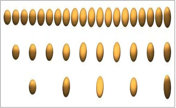
Example 5. It is well-known (see for instance [1] and [3]) that the space of posi-tive definite symmetric matrices is a Riemannian symmetric space. Moreover, it is also a Hadamard manifold with exponential map (globally) given by Expp(v) =
p1/2exp(p−1/2vp−1/2)p1/2. Choosingf =Expand applying 2 rounds of qubic B-spline
[image:10.612.125.460.328.535.2]geodesic subdivision we get the following figure. Note that each ellipsoid represents a positive definite symmetric matrix.
Figure 1: Subdivision in the space of positive matrices
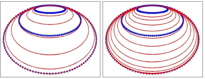
Example 6. In the following we consider as a prominent example of a Hilbert manifold the loop space of R2 and apply qubic B-spline geodesic subdivision to the polygon p consisting of loops p1, p2 and p3 through a fixed pint. Figure 2 shows the result
Figure 2: Subdivision in the loop space
5.Conclusions and remarks
We have established the notion of analogues of a linear subdivision operating on manifold-valued data. Furthermore we have investigated smoothness properties of such subdivision schemes. Particulrly, we have shown that if the linear scheme enjoys C2 smoothness and its derived schemes up to order 3 satisfy certain boundedness
inequalities, then the nonlinear analogues one is also C2.
Acknowledgement:The author wish to thank professor J. Wallner and P. Grohs for their helpful discussions.
This work was supported by Grant No. 18575 of the Austrian Science Fund (FWF).
References
[1] P. T. Fletcher and S. Joshi,Principal Geodesic Analysis on Symmetric Spaces: Statistics of Diffusion Tensors,2004, Computer Vision and Mathematical Methods in Medical and Biomedical Image Analysis, M. Sonka and I. Kakadiaris and J. Kybic (editors), Lecture Notes in Computer Science, number 3117, pp. 87-98.
[2] P. Grohs,Smoothness of multivariate subdivision in Lie groups, Tech. Report, TU Graz, 2007, http://dmg.tuwien.ac.at/grohs/inter.pdf.
[4] E. Nava-Yazdani, A general class of nonlinear univariate subdivision algo-rithms and their C2 smoothness, Geometry preprint, TU Graz, August 2007.
[5] I. Ur Rahman, I. Drori, V. C. Stodden, D. L. Donoho, and P. Schr¨oder, Multi-scale representations for manifold-valued data, MultiMulti-scale Modeling and Simulation, 4 (2005), pp. 1201–1232.
[6] J. Wallner,Smoothness analysis of subdivision schemes by proximity, Constr. Approx., 24 (2006), pp. 289–318.
[7] J. Wallner and N. Dyn, Convergence and C1 analysis of subdivision schemes
on manifolds by proximity, Comput. Aided Geom. Design, 22 (2005), pp.593–622. [8] J. Wallner and P. Grohs, Log-exponential analogues of univariate subdivision schemes in Lie groups and their smoothness properties, Tech. Report, TU Graz, 2007, http://www.geometrie.tugraz.at/wallner/grvar.pdf.
[9] J. Wallner, E. Nava Yazdani and P. Grohs,Smoothness properties of Lie groups subdivision schemes, SIAM Journal of Multiscale Modeling and Simulation, volume 6 (2007), pp. 493-505.
[10] G. Xie and T. P. Y. Yu,Smoothness equivalence properties of manifold-valued data subdivision schemes based on the projection approach, SIAM J. Numer. Anal., Preprint, http://www.math.drexel.edu/∼tyu/Papers/SmoothnessEquiv.pdf
Author:
Esfandiar Nava-Yazdani Institute of Geometry
Graz University of Technology Kopernikusgasse 24/IV
8010 Graz/Austria