AN INTRODUCTION TO DISTANCE ID/I MAGIC GRAPHS | O'Neal | Journal of the Indonesian Mathematical Society 22 370 1 PB

(1)

Special Edition (2011), pp. 89–107.

AN INTRODUCTION TO DISTANCE D MAGIC

GRAPHS

Allen O’Neal

1

, Peter J. Slater

2

1_{Mathematical Sciences Department, University of Alabama Huntsville, AL,}

USA 35899 [email protected]

2_{Mathematical Sciences Department and Computer Sciences Department,}

University of Alabama Huntsville, AL, USA 35899 [email protected] and

[email protected]

Abstract. For a graph G of order |V(G)| = n and a real-valued mapping f :V(G)→ R_{, if} _S _⊂_V₍_G_{) then} _f₍_S_{) =} P

w∈Sf(w) is called the weight ofS

underf. When there exists a bijectionf :V(G)→[n] such that the weight of all open neighborhoods is the same, the graph is said to be 1-vertex magic, or Σ la-beled. In this paper we generalize the notion of 1-vertex magic by defining a graph Gof diameter dto beD-vertex magic when for D ⊂ {0,1, . . . , d}, we have that

P

u∈N_D(v)f(u) is constant for allv∈V(G). We provide several existence criteria for graphs to beD-vertex magic and use them to provide solutions to several open problems presented at the IWOGL 2010 Conference. In addition, we extend the no-tion of vertex magic graphs by providing measures describing how close a non-vertex magic graph is to being vertex magic. The general viewpoint is to consider how to assign a setWof weights to the vertices so as to have an equitable distribution over theD-neighborhoods.

Key words: Graph Labeling, vertex magic, Σ labeling, distance magic graphs, neigh-borhood sums.

2000 Mathematics Subject Classification: 05C78.

(2)

Abstrak. Untuk suatu grafGberorde|V(G)|=ndan sebuah pemetaan bernilai riilf :V(G)→R_{, jika}_S_⊂_V₍_G_{) maka}_f₍_S_{) =}P

w∈Sf(w) disebut bobot dariS

olehf. Ketika terdapat sebuah bijeksif :V(G)→[n] sehingga bobot dari semua himpunan buka adalah sama, graf dikatakan menjadi ajaib 1-titik, atau dilabelkan Σ. Pada paper ini kami memperumum ide dari ajaib 1-titik dengan pendefinisian sebuah grafGberdiameterdmenjadi ajaib D-titik jika untukD ⊂ {0,1, . . . , d}, kita mempunyai bahwaPu∈N_D(v)f(u) adalah konstan untuk semua v ∈ V(G). Kami memberikan beberapa kriteria keberadaan untuk graf-graf menjadi ajaibD -titik dan menggunakan mereka untuk memberikan solusi beberapa masalah terbuka yang disajikan di konferensi IWOGL 2010. Lebih jauh, kami memperluas ide graf-graf ajaib titik dengan pemberian ukuran-ukuran yang menggambarkan seberapa dekat sebuah graf ajaib bukan titik mnejadi ajaib titik. Titik pandang umum adalah bagaimana untuk menyatakan suatu himpunanW dari bobot-bobot ke titik-titik sehingga mempunyai suatu distribusi yang seimbang sepanjang ketetanggaan-D.

Kata kunci: Pelabelan graf, ajaib titik, pelabelan Σ, graf ajaib jarak, jumlah kete-tanggaan.

1. Introduction

One type of graph labeling problem involves labeling the vertices of a graph Gand then computing a value g(v) for each v ∈V(G), whereg(v) is determined by the labels on some set S(v) ⊂ V(G). Properties of the graph can be defined based on the permissible sets of values that are produced by the set of labelings

{g(v) : v ∈ V(G)}. For example, for a graph G = (V, E) of order n, one can define a bijectionf :V(G)→ {1,2, . . . , n}and then for each vertex, sum the labels in its open (or closed) neighborhood. One case that has been studied is the case where the set of resulting open neighborhood sums are all equal. Vilfred [9] called such a labeling a Σ labeling and any graph for which such a labeling exists a Σ graph. Miller et al. [2] referred to such a labeling as a 1-vertex magic labeling. More recently Sugeng et al. [8] have referred to such a labeling as a distance magic labeling. When the closed neighborhood sums are all equal, Beena [1] has referred to the labeling as a Σ′

labeling and the graph as a Σ′

graph. Each of these works has focused on either the open or closed neighborhood case.

(3)

Each of the works mentioned has focused on the existence/non-existence of labelings for particular graphs. We extend the existence question and define mea-sures that can be used to classify how close a particular graph is to being distance magic. For example, when a graph is not Σ labeled, we measure how close is it to being Σ labeled.

2. Definitions

In this section we give our definitions, including that of a graphGbeing D -vertex magic for an arbitrary setD⊂ {0,1, . . . , diam(G)}, and we illustrate these definitions for the House graphHin Figure 1(a). Throughout the paper we assume graphGhas order|V(G)|=n, diameterdiam(G) =d, and thatD⊂ {0,1, . . . , d}.

Definition 2.1. For v ∈ V(G), the D-neighborhood of v, denoted by ND(v), is

defined as ND(v) ={u∈V(G) :d(v, u)∈D}.

IfD ={1}, then ND(v) is the open neighborhood of the vertex v. We will

adopt the notation thatN(v) =N{1}(v). We taked(v, v) = 0. Thus, ifD={0,1},

thenND(v) is the closed neighborhood of the vertexv. We will adopt the notation

that N[v] =N{0,1}(v).

Definition 2.2. Let V(G) ={v1, v2, . . . , vn}. The distance D adjacency matrix,

denoted byAD= [ai,j], is defined to be then×nbinary matrix withai,j = 1if and

only ifd(vi, vj)∈D.

IfD={1}, then AD=A is the adjacency matrix ofGin the usual fashion.

IfD={0,1}, thenAD=A+I=N whereIis then×nidentity matrix, andN is

called the closed neighborhood matrix ofG. Also note that for anyD⊂ {0,1, . . . , d}

we have thatAD is symmetric.

Definition 2.3. Graph G is defined to be (D, r)-regular if for all v ∈ V(G), P

u∈ND(v)1 =r, that is, all D-neighborhoods have the same cardinality.

Note that for a graphGto be ({1}, r)-regular or, equivalently, ({0,1}, r+ 1)-regular corresponds toGbeingr-regular.

Definition 2.4. Let W ={w1, w2, . . . , wn} ⊂ R be a set (or, more generally, a

multiset) of real numbers referred to as weights. For a bijection f : V(G) → W

and a subset S ⊂ V(G), the weight of S under f, denoted by f(S), is defined as

f(S) =P_v_∈_Sf(v).

(4)

multiset). For a bijection f :V(G)→W, we define the D-neighborhood sum off,

denoted byN S(f;D), asN S(f;D) =max{f(ND(v))|v∈V(G)}.

When D = {1} we will by convention shorten the notation to N S(f) = N S(f;{1}). Similarly, whenD={0,1}we will by convention shorten the notation toN S[f] =N S(f;{0,1}).

multiset). The W-valued D-neighborhood sum of G, denoted by N SW(G;D), is

defined as N SW(G;D) =min{N S(f;D)|f :V(G)→W is a bijection}.

WhenD ={1} we will adopt the previous convention and shorten the no-tation to N SW(G) = N SW(G;{1}). Likewise, when D = {0,1} we shorten the

notation toN SW[G] =N SW(G;{0,1}).

For a graphG= (V, E) of order|V(G)|=nwe are generally interested in the set of weightsW = [n] ={1,2, . . . , n}. When this is the case, we will by convention shorten the notation to N S(G;D) =N SW(G;D). So for the open neighborhood

sum case (that is, when D ={1}) with weight setW = [n], our notation will be N S(G) =N SW(G;{1}). For the closed neighborhood sum case (that is, whenD=

{0,1}) with weight setW = [n], our notation will be N S[G] =N SW(G;{0,1}).

By following these conventions, our notation matches what has been introduced by Schneider and Slater [6, 7].

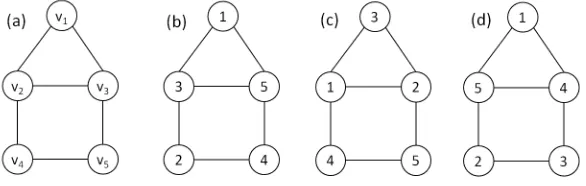
Example 2.7. Consider the graph H= (V, E)in Figure 1(a) which has diameter

2. We claim thatN S(H) = 8,N S[H] = 11, andN S(H;{2}) = 6.

Figure 1. Minimax and maximin labelings of House graphH

To see thatN S(H) = 8, consider thatN(v2)∪N(v4) =V(H)and N(v2)∩

N(v4) =∅_{. Hence, for any bijection}_f _:_V₍_H₎_→_[5]_{, we must have that}_f₍_N₍_v2₎₎₊

f(N(v4)) = 15. It follows that one of{f(N(v2)), f(N(v4))}is greater than or equal

to 8. From this we have that N S(H) ≥ 8. The bijection shown in Figure 1(b)

(5)

To see thatN S[H] = 11, letf :V(H)→[5]be an arbitrary bijection. Notice

that one of {f(v4), f(v5)} is no more than 4. If f(v4) ≤ 4, then f(N[v3]) =

15−f(v4)≥11. Similarly, if f(v5)≤4, then f(N[v2]) = 15−f(v5)≥11. Thus

N S[H]≥11. The bijection shown in Figure 1(c) demonstrates that N S[H]≤11.

Therefore,N S[H] = 11.

Finally, to see that N S(H;{2}) = 6, let f : V(H) → [5] be an arbitrary

bijection. Notice that iff(v1) = 5orf(v2) = 5, thenf(N{2}(v5)) =f(v1)+f(v2)≥

6. If f(v3) = 5, then f(N{2}(v4)) =f(v1) +f(v3)≥6. If f(v4) = 5 orf(v5) = 5,

thenf(N{2}(v1)) =f(v4) +f(v5)≥6. ThusN S(H;{2})≥6. The bijection shown

in Figure 1(b) demonstrates thatN S(H;{2})≤6. Therefore,N S(H;{2}) = 6.

Next we consider maximizing the minimum weight of aD-neighborhood.

multiset). For a bijection f :V(G)→W, we define the lower D-neighborhood sum

of f, denoted byN S−₍_f_;_D₎_{, as}_{N S}−₍_f_;_D_{) =}_min_{_f₍_N

D(v))|v∈V(G)}.

When D = {1} we will by convention shorten the notation to N S−₍_f_{) =}

N S−₍_f_;_D_{). Similarly, when}_D₌_{₀_,₁_}_{we will by convention shorten the notation}

toN S−_[_f_{] =}_{N S}−₍_f_;_D_).

multiset). The W-valued lower D-neighborhood sum of G, denoted by N SW−(G;D),

is defined as N S−_W(G;D) =max{N S−₍_f_;_D₎_|_f _:_V₍_G₎_→_W _{is a bijection}_}_.

WhenD ={1} we will adopt the previous convention and shorten the no-tation to N S_W−(G) = N S_W−(G;D). Likewise, when D = {0,1} we shorten the notation toN S_W−[G] =N S_W−(G;D).

When our weight set isW = [n] ={1,2, . . . , n}, we will again adopt the no-tationN S−₍_G_;_D_{) =}_{N S}−

W(G;D). So, for the open neighborhood sum case, where

D ={1}, with weight setW = [n], our notation will beN S−₍_G_{) =}_{N S}− W(G;D).

For the closed neighborhood sum case, whereD={0,1}, with weight setW = [n], our notation will be N S−_[_G_{] =}_{N S}−

W(G;D). By following these conventions, our

notation matches what has been introduced by O’Neal and Slater [3].

Example 2.10. Consider the graph H= (V, E) from Figure 1(a). We claim that

N S−(H) = 7,N S−[H] = 9, andN S−(H;{2}) = 4.

To see that N S−₍_H_{) = 7}_{, again notice that} _N₍_v2₎_∪_N₍_v4_{) =} _V₍_H₎ _and

N(v2)∩N(v4) = ∅_{. Hence for any bijection} _f _: _V₍_H₎ _→_[5] _{we must have that}

f(N(v2)) +f(N(v4)) = 15. It follows that one of{f(N(v2)), f(N(v4))}is less than

or equal to 7; hence we have thatN S−₍_H₎_≤₇_{. The bijection shown in Figure 1(b)}

demonstrates thatN S−₍_H₎_≥₇_{. Therefore, we conclude that}_{N S}−₍_H_{) = 7}_.

Figure 1(d) demonstrates that N S−_[_H_] _≥₉_{. If there exists a bijection} _f _:

(6)

5. However, this would imply that one of{f(N[v4]), f(N[v5])} is no more than 9.

Therefore, such a bijection does not exist, and we conclude thatN S−_[_H_{] = 9}_.

Finally, we show thatN S−₍_H_;_{₂_}_{) = 4}_{. Consider that one of}_{_f₍_v4₎_{, f}₍_v5₎_}

is less than or equal 4. If f(v4)≤4, then f(N{2}(v3)) =f(v4)≤4. If f(v5)≤4,

then f(N{2}(v2)) =f(v5)≤4. Hence N S−(H;{2})≤4. The bijection shown in

Figure 1(c) demonstrates thatN S−₍_H_;_{₂_}₎_≥₄_{. Therefore,}_{N S}−₍_H_;_{₂_}_{) = 4}_.

Consider the closed neighborhood sumN S[H] and the lower closed neighbor-hood sum N S−_[_H_{]. For bijection} _f _{in Figure 1(c), we have closed neighborhood}

sums{6,10,11,10,11} achievingN S[H] = 11 =f(N[v3]) = f(N[v5]). Note that f(N[v1]) = 6. For bijection g of Figure 1(d), we have closed neighborhood sums

{10,12,13,10,9}withN S−_[_H_{] =}_g₍_N_[_v5_{]) = 9. Is there a bijection}_h_:_V₍_G₎_→_[5]

that simultaneously achievesN S[H] andN S−_[_H_{]? Our third measure of}

equitabil-ity considers the range of values in{f(ND(v1)), . . . , f(ND(vn))}.

Definition 2.11. Let W ={w1, w2, . . . , wn} ⊂R be a set (or, more generally, a

multiset). For a bijection f :V(G)→W, we define the D-neighborhood spread of

f, denoted byN Ssp₍_f_;_D₎_{, as}_{N S}sp₍_f_;_D_{) =}_{N S}₍_f_;_D₎₋_{N S}−₍_f_;_D₎_.

As before, when D = {1} we will by convention shorten the notation to N Ssp₍_f_{) =}_{N S}sp₍_f_;_D_{). Similarly, when}_D₌_{₀_,₁_}_{we will by convention shorten}

the notation toN Ssp_[_f_{] =}_{N S}sp₍_f_;_D_).

Definition 2.12. Let W = {w1, w2, . . . , wn} ⊂ R be a set (or, more generally,

a multiset). The W-valued D-neighborhood spread of G, denoted by N S_Wsp(G;D),

is defined as N S_Wsp(G;D) = min{N S(f;D)−N S−₍_f_;_D₎_| _f _: _V₍_G₎ _→ _W _{is a}

bijection}.

WhenD ={1} we will adopt the previous convention and shorten the no-tation to N S_Wsp(G) = N S_Wsp(G;D). Likewise, when D = {0,1} we shorten the notation toN S_Wsp[G] =N S_Wsp(G;D).

When our weight set is W = [n] = {1,2, . . . , n}, we will again shorten the notation to N Ssp₍_G_;_D_{) =} _{N S}sp

W(G;D). So for the open neighborhood sum

case, where D ={1}, with weight set W = [n], our notation will be N Ssp₍_G_{) =}

N SWsp(G;D). For the closed neighborhood sum case, whereD={0,1}, with weight

setW = [n], our notation will beN Ssp[G] =N SWsp(G;D). By following these

con-ventions, our notation matches what has been introduced by O’Neal and Slater [3].

Definition 2.13. GraphGis said to be D-vertex magic, or equivalently D-distance

magic, if there exists a bijection f :V(G)→[n] and a constantc such that for all

v∈V(G), P u∈N_D(v)

f(u) =c, that is,f has D-neighborhood spread zero.

(7)

Similarly, for a graph with diameterdand for 0< i < d, the graph isi-vertex magic if and only if the graph is D-vertex magic with D={i}.

For any graph G = (V, E) with order n, N S(G), N S−₍_G_{), and} _{N S}sp₍_G₎

are each measures of how close the graph is to being 1-vertex magic (Σ labeled). More generally, for D ⊂ {0,1, . . . , d} where d is the diameter of G, N S(G;D), N S−₍_G_;_D_{), and}_{N S}sp₍_G_;_D_{) give us measures of how close}_G_{is to being}_D_-vertex

magic.

Example 2.14. For the graph H from Figure 1(a), we claim that N Ssp₍_H_{) = 1}_,

N Ssp_[_H_{] = 4}_{, and}_{N S}sp₍_H_;_{₂_}_{) = 4}_.

Since N S(H) = 8 and N S−₍_H_{) = 7}_{, clearly} _{N S}sp₍_H₎ _≥₁_{. The bijection}

shown in Figure 1(b) demonstrates thatN Ssp₍_H₎_≤₁_{. Therefore,} _{N S}sp₍_H_{) = 1}_.

The bijection from Figure 1(b) also demonstrates thatN Ssp_[_H_]_≤₄_{. Assume}

there exists a bijection f : V(H)→ [5] such thatN Ssp_[_f_]_≤₃_{. Since} _f₍_N_[_v2_])₋

f(N[v1]) = f(v4), we must have that f(v4) ≤ 3. Similarly, we must have that

f(v5)≤3. Hence, one of {f(v4), f(v5)} is less than or equal 2. Iff(v4)≤2, then

f(N[v3])≥13. Iff(v5)≤2, thenf(N[v2])≥13. But since N S−_[_H_]_≤₉_{, we have}

that N Ssp_[_f_]_≥₄_{, which is a contradiction. Therefore,}_{N S}sp_[_H_{] = 4}_.

Finally, notice that the bijection from Figure 1(b) also demonstrates that

N Ssp₍_H_;_{₂_}₎ _≤ ₄_{. Assume there exists a bijection} _f _: _V₍_H₎ _→ _[5] _{such that}

N Ssp₍_H_;_{₂_}₎_≤₃_{. In this case}_f₍_N

{2}(v1))−f(N{2}(v2)) =f(v4)≤3. Similarly,

f(N{2}(v1))−f(N{2}(v3)) =f(v5)≤3. Thus, one of{f(v4), f(v5)}is less than or

equal 2. If f(v4)≤2, then we have f(N{2}(v3)) = f(v4)≤2. If f(v5) ≤2, then

we havef(N{2}(v2)) =f(v5)≤2. In either case, since N S(H;{2})≥6, we have

that N Ssp₍_f_;_{₂_}₎_≥₄_{, which is a contradiction. Therefore,}_{N S}sp₍_H_;_{₂_}_{) = 4}_.

These examples demonstrate that there are graphs whereN Ssp_[_G_]_{> N S}_[_G_]₋

N S−_[_G_{]. Where this is the case, there cannot be a single bijection that achieves}

both N S[G] and N S−_[_G_{]. We note that there are graphs such that}_{N S}sp₍_G₎ _>

N S(G)−N Ssp₍_G_).

Also notice that for the graphH in these examples, we had thatN S[H] + N S−₍_H_;_{₂_}_{) =} n(n+1)

2 = 15 = N S−[H] +N S[H;{2}] and that N Ssp[H] = N Ssp₍_H_;_{₂_}_{). This result was not a coincidence, and the more general result}

will be proven in the next section in Theorem 3.1.

Example 2.15. For graph G and weight set W = {w1, w2, . . . , wn}, if D =

{0,1,2, . . . , d}, then it is trivially true that N SW[G;D] =N SW−[G;D] = Pn

i=1wi

and that N S_Wsp[G;D] = 0. Since the diameter of the graph H in the previous

ex-ample is 2, when D ={0,1,2}, we have that N S[H;D] = N S−_[_H_;_D_{] = 15} _and

N Ssp_[_H_;_D_{] = 0}_.

3. Existence Theorems forD-vertex Magic Graphs

Theorem 3.1. Let D ⊂ {0,1, . . . , d} and let D#₌_{₀_,₁_{, . . . , d}_{} −}_D_{. Then} _G _is

(8)

Proof. Let f : V(G) → [n] be a bijection and c a constant such that for G is D#_{-vertex magic. Since the set} _D _{was arbitrary, this suffices to prove the}

converse as well.

Corollary 3.4. Let G= (V, E)be any regular graph. For the closed neighborhood

matrix N, if N−1 _{exists, then} _G _{is not} _{₀_,₁_}_{-vertex magic, that is,} _G _{is not} _Σ′

labeled.

In Miller et al. [2] it was proved that there does not exist a {1}-vertex r-regular graph for odd r. In the next result we extend this idea to arbitrary neighborhood sets. which is a contradiction. Hence, no such bijectionf exists, and therefore,Gis not

D-vertex magic.

Corollary 3.6. If Gis(D, r)regular with rodd, thenGis not D-vertex magic.

Proof. Since 0 ∈/ D, all the elements on the diagonal ofAD are 0. Since AD is

(9)

Since r is odd, AD has an odd number r of 1’s in each row, and we must haven

even. Thus the result follows from Theorem 3.5.

Corollary 3.7. There does not exist a graph of even order that is both{1}-vertex

magic and {0,1}-vertex magic. That is, there does not exist a graph of even order

that is bothΣ labeled andΣ′ labeled.

We will now use these theoretical results to provide solutions to problems that were posed at the 2010 IWOGL Conference. For each of the following examples, the question was posed whether there existed {d}-vertex magic labelings of the graphs, wheredis the diameter of the graph.

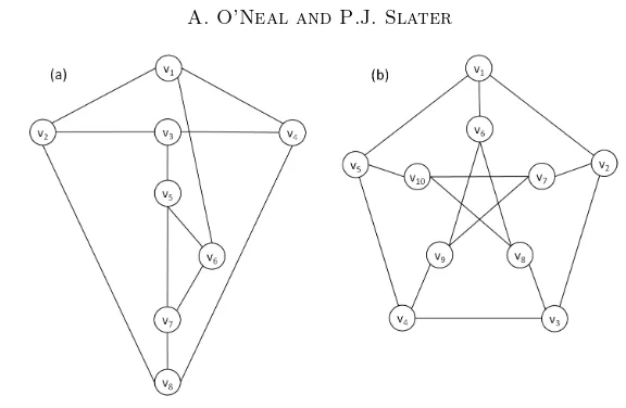
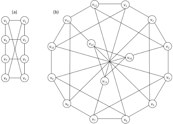
Example 3.8. Consider the graph G1 in Figure 2(a) which has order 8 and

di-ameter 2. G1 is regular of degree 3. Let f :V(G1)→ [8]be any bijection. Since

f(N(v1)) = f(v2) +f(v4) +f(v6) 6= f(v2) +f(v4) +f(v7) = f(N(v8)), G1 is

not {1}-vertex magic, or equivalently, G1 is not Σ labeled. By Theorem 3.1, G1

is not {0,2}-vertex magic. Since f(N[v2]) = f(v1) +f(v2) +f(v3) +f(v8) 6=

f(v1) +f(v3) +f(v4) +f(v8) =f(N[v4]),G1is not{0,1}-vertex magic, or

equiva-lently,G1is notΣ′−labeled. SinceG1 is not{0,1}-vertex magic, by Theorem 3.1,

G1 is not{2}-vertex magic.

Making use of Theorem 3.2, we could also consider the closed neighborhood

matrixN and notice thatdet(N) =−16= 06 . HenceG1 is not{0,1}-vertex magic.

By Theorem 3.1 it follows thatG1 is not {2}-vertex magic. The adjacency matrix

for G1 is singular, so we cannot apply Theorem 3.2 in that case. However since

G1 has even order and is ({1},3) regular, we can apply Theorem 3.5 to conclude

that G1 is not{1}-vertex magic, and then apply Theorem 3.1 to conclude thatG1

is not {0,2}-vertex magic.

Example 3.9. Consider the Petersen Graph P in Figure 2(b). The order of P is

10, the diameter of P is 2, and P is 3-regular. det(A) = 48 6= 0 where A is the

adjacency matrix forP. HenceP is not {1}-vertex magic by Theorem 3.2, and by

Theorem 3.1, P is not {0,2}-vertex magic. We could have also used Theorem 3.5

to conclude thatP was not {1}-vertex magic.

We havedet(N) = 1286= 0whereN is the closed neighborhood matrix forP.

So by Theorem 3.2, P is not {0,1}-vertex magic, and then by Theorem 3.1, P is

not {2}-vertex magic.

Example 3.10. Consider the graph G2 in Figure 3(a) which has order 8 and

diameter 2. G2 is regular of degree 3. Let f : V(G2) → [8] be any bijection.

If G2 is {1}-vertex magic, then f(N(v3)) = f(N(v6)). However, f(N(v3)) =

f(v2) +f(v4) +f(v7) 6= f(v2) +f(v5) +f(v7) = f(N(v6)). Hence, G2 is not

(10)

Figure 2. 3-Regular graphG1 and Petersen graphP

IfG2 is{0,1}-vertex magic, then by O’Neal and Slater[3]we know that each

closed neighborhood sum must equal 18. Hence f(N[v8]) =f(v1) +f(v4) +f(v7) +

f(v8) = 18 and f(N[v2]) = f(v1) +f(v2) +f(v3) +f(v6) = 18. It follows that

2f(v1) +f(v2) +f(v3) +f(v4) +f(v6) +f(v7) +f(v8) = 36. But we also have that

f(v1) +· · ·+f(v8) = 36. Subtracting we get that forG2to be {0,1}-vertex magic,

we must have f(v1)−f(v5) = 0, which would be a contradiction. Hence,G2 is not

{0,1}-vertex magic. From Theorem 3.1 it follows thatG2 is not{2}-vertex magic.

Making use of Theorem 3.2, we could also consider the adjacency matrixA

and notice that det(A) = −3 = 06 . Hence G2 is not {1}-vertex magic, and by

Theorem 3.1,G2is not{0,2}-vertex magic. Alternatively, sinceG2has even order

8 and is ({1},3)regular, by Theorem 3.5, G2 is not {1}-vertex magic. The closed

neighborhood matrix N for G2 is singular, so we cannot apply Theorem 3.1 to

conclude thatG2 is not{0,1}-vertex magic.

Proposition 3.11. Let Mn be a Mobius Ladder of order 2n with n > 2. Mn is

neither{1}-vertex magic nor{0,1}-vertex magic.

Proof. Notice that if n > 2, then there exists vertices u, v ∈ V(Mn) such that

|N[u]△N[v]|= 1or2, where△ denotes symmetric difference. Hence, by Theorem 9 Beena [1],Mn is not{0,1}-vertex magic. SinceMn has even order and is regular

of degree 3, by Theorem 3.5,Mn is not{1}-vertex magic. Note that ifn= 2, then

M2=K4 and henceM2is{0,1}-vertex magic but not{1}-vertex magic.

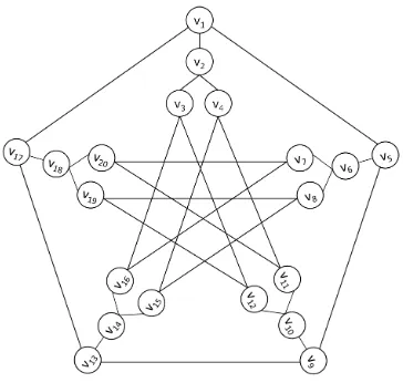
Example 3.12. Consider the graph G3 in Figure 3(b) which has order 15 and

diameter 2. G3 is regular of degree 4. det(A) = 12806= 0 so by Theorem 3.2 G3

is not {1}-vertex magic, and thus by Theorem 3.1, G3 is not{0,2}-vertex magic.

(11)

Figure 3. Mobius ladderG2 and graphG3

Theorem 3.2, G3 is not {0,1}-vertex magic. Hence by Theorem 3.1, G3 is not

{2}-vertex magic.

Example 3.13. Consider the graph G4 in Figure 4 which has order 24 and

di-ameter 2. G4 is regular of degree 5. det(A) = 6,298,560 6= 0 and so by Theorem

3.2, G4 is not{1}-vertex magic, and thus by Theorem 3.1, G4 is not {0,2}-vertex

magic. We could have also used Theorem 3.5 to conclude that G4 was not {1}

-vertex magic. det(N) = 34,012,2246= 0whereN is the closed neighborhood matrix

of G4, and so by Theorem 3.2, G4 is not {0,1}-vertex magic. Hence by Theorem

3.1, G4 is not{2}-vertex magic.

Example 3.14. Consider the graph G5 in Figure 5 which has order 20 and

di-ameter 3. G5 is regular of degree 3. det(A) = 12 6= 0 and so by Theorem 3.1,

G5 is not {1}-vertex magic, and thus by Theorem 3.1, G5 is not {0,2,3}-vertex

magic. We could also apply Theorem 3.5 to achieve the same result. Similarly

det(A{1,2}) = 20,736 6= 0 and we can conclude that G5 is neither {1,2}-vertex

magic nor {0,3}-vertex magic. Again Theorem 3.5 could be used to achieve this

same result. det(A{0,2}) =−47,0686= 0 soG5 is neither {0,2}-vertex magic nor

{1,3}-vertex magic. A{0,1} andA{0,1,2} are both singular.

We do have that rank(A{0,1}) = 19 and so dim(N(A{0,1})) = 1. Further

y = [−1,3,−1,−1,−1,3,−1,−1,−1,3,−1,−1,−1,3,−1,−1,−1,3,−1,−1]T _{is a}

(12)

Figure 4. 5-Regular graphG4 of order 24 and diameter 2

system A{0,1}x = c−→1, any solution to the non-homogeneous system must equal

ay +z for some constant a. Since no value of a produces a solution that is a

permutation of [1,2, . . . ,20]T_{, we can conclude that} _G₅ _{is not}_{₀_,₁_}_{-vertex magic,}

and thus by Theorem 3.1, G5 is not {2,3}-vertex magic.

We also have that rank(A{0,1,2}) = 19. Using the null space basis vector

y = [0,0,1,−1,0,0,1,−1,0,0,1,−1,0,0,1,−1,0,0,1,−1]T and the same logic, we

can conclude thatG5 is not{0,1,2}-vertex magic, and hence,G5is not{3}-vertex

magic.

(13)

4. General Results

In Section 2 we introduced terminology that allows us to make a statement about how close any graph is to being vertex magic. In this section we provide some basic results that build upon the terminology introduced.

(14)

n P i=1

wi+g(ND(u)) = N Ssp(g;D). Consider the bijection f : V(G) → W where

N S_Wsp(G;D) = N Ssp₍_f_;_D₎_. _{Since the relationship above holds for the arbitrary}

bijection g, we mush have that N S_Wsp(G;D) = N Ssp₍_f_;_D_{) =} _{N S}sp₍_f_;_D#_{) =} N SW(G;D#). The last equality must hold, for if there exists a bijection h :

V(G) → W such that N Ssp(h;D#) < N Ssp(f;D#), then N Ssp₍_h_;_D₎_{< N S}sp₍_f_;_D_{), but this would be a contradiction.}

Corollary 4.2. Let D⊂ {0,1, . . . , d}andD#₌_{₀_,₁_{, . . . , d}_{} −}_D_{. Then}

(i) For a bijectionf :V(G)→[n] and a vertex v∈V(G),N S(f;D) =f(ND(v))

if and only if N S−₍_f_;_D#_{) =}_f₍_N

D#(v));

(ii) For a bijection f : V(G) → [n], N S(G;D) = N S(f;D) if and only if

N S−₍_G_;_D#_{) =}_{N S}−₍_f_;_D#₎_;

(iii)N S(G;D) +N S−₍_G_;_D#_{) =}n(n+1)

2 ; and

(iv)N Ssp₍_G_;_D_{) =}_{N S}sp₍_G_;_D#₎_.

Example 4.3. For the graph H from Figure 1(a), we showed in Example 2.7 that N S[H] = 11, and we showed in Example 2.10 that N S−₍_H_;_{₂_}_{) = 4}_.

No-tice that N S[H] +N S−₍_H_;_{₂_}_{) =} 5(6)

2 = 15. In Example 2.10 we showed that

N S−_[_H_{] = 9}_{, and in Example 2.7 we showed that} _{N S}₍_H_;_{₂_}_{) = 6}_{. Notice that}

N S−_[_H_{] +}_{N S}₍_H_;_{₂_}_{) = 15}_{. In Example 2.14 we showed that} _{N S}sp_[_H_{] = 4} _and that N Ssp₍_H_;_{₂_}_{) = 4}_.

Example 4.4. For the graph H from Figure 1(a), we showed in Example 2.7 that N S(H) = 8, in Example 2.10 that N S−(H) = 7, and in Example 2.14 that N Ssp₍_H_{) = 1}_{. Using Corollary 4.2 we conclude that} _{N S}₍_H_;_{₀_,₂_}_{) = 8}_,

N S−₍_H_;_{₀_,₂_}_{) = 7}_{, and that}_{N S}sp₍_H_;_{₀_,₂_}_{) = 1}_.

The following corollary was proven as Theorem 1 by O’Neal and Slater [3] and is included here for completeness.

Corollary 4.5. Let GC _{be the complement of} _G_{. Let} _W ₌_{_{w1, w2, . . . , w} n} ⊂R be a set (or, more generally, a multiset). Then

(i)N SW(G;{0,1}) +N SW−(GC;{1}) =

n P i=1

wi=N SW(G;{1}) +N SW−(GC;{0,1}),

and

(ii) N S_Wsp(G;{0,1}) =N Ssp_W(GC_;_{₁_}₎_.

Proof. Notice that if we take D = {0,1} and D# ₌_{₂_,₃_{, . . .}_}_{, then for every} v∈V(G),ND#(v) inGcontains exactly the same set of vertices as theN_{₁_}(v) in

(15)

Corollary 4.6. Let GC _{be the complement of} _G_{. Then}

(i)N S(G;{0,1})+N S−₍_GC_;_{₁_}_{) =}n(n+1)

2 =N S(G;{1})+N S−(GC;{0,1}), and

(ii) N Ssp₍_G_;_{₀_,₁_}_{) =}_{N S}sp₍_GC_;_{₁_}₎_.

Example 4.7. Consider again the graphH from Figure 1(a). The complement of

H is the path P5. Using Corollary 4.6 and the results from previous examples we

can make the following observations: (i)N S[P5] = 15−N S−₍_H_{) = 8}_. (ii)N S−_[_P5_{] = 15}₋_{N S}₍_H_{) = 7}_.

(iii)N Ssp_[_P5_{] =}_{N S}sp₍_H_{) = 1}_.

(iv)N S(P5) = 15−N S−_[_H_{] = 6}_. (v)N S−₍_P5_{) = 15}₋_{N S}_[_H_{] = 4}_. (vi)N Ssp₍_P5_{) =}_{N S}sp₍_H_{) = 4}_.

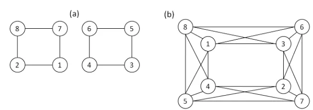
Example 4.8. Consider the graphG6 in Figure 6 whose complement isC6. From

O’Neal and Slater[4]we know thatN S(C6) = 9,N S−₍_C6_{) = 5}_{, and}_{N S}sp₍_C6_{) = 4}_.

One can also show that N S[C6] = 11, N S−_[_C6_{] = 10}_{, and} _{N S}sp_[_C6_{] = 1}_{. Using}

Corollary 4.6 we can conclude thatN S(G6) = 11,N S−₍_G_{6) = 10}_,_{N S}sp₍_G_{6) = 1}_,

N S[G6] = 16,N S−_[_G_{6] = 12}_{, and}_{N S}sp_[_G_{6] = 4}_{. The labeling for the open} neigh-borhood case is shown in Figure 6(a) and the labeling for the closed neighneigh-borhood case is shown in Figure 6(b).

Figure 6. Labelings of G6 showing N S(G6) = 11, N S−(G6) = 10,N Ssp₍_G_{6) = 1,}_{N S}_[_G_{6] = 16,}_{N S}−_[_G_{6] = 12,}_{N S}sp_[_G_{6] = 4}

Corollary 4.9. A graph G is Σ labeled if and only if its complement GC _is _Σ′ labeled.

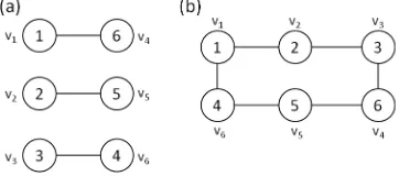
Example 4.10. From O’Neal and Slater [4]we know that a 2-regular graph is Σ

labeled if and only if it is the union of 4 cycles. Figure 7(a) shows aΣlabeling of the

union of two 4 cycles. Figure 7(b) shows theΣ′ labeling of the graph’s complement.

Corollary 4.11. Define the graphH = (V, E)byV(H) =V(G)and for allu, v∈

V(G)letuv∈E(H)if and only if d(u, v)∈D. Then:

(i)N S(G;{0} ∪D) =N S[H],

(16)

Figure 7. Σ labeling of the union of 2C4’s, and Σ′ labeling of its complement

(iii)N Ssp₍_G_;_{₀_{} ∪}_D_{) =}_{N S}sp_[_H_]_.

(iv)N S(G;D) =N S(H).

(v) N S−₍_G_;_D_{) =}_{N S}−₍_H₎_.

(vi)N Ssp₍_G_;_D_{) =}_{N S}sp₍_H₎_.

Proof. Notice that for any choice ofD, for allv∈V(G), theND(v) inGcontains

exactly the same set of vertices as theN{1}(v) inH.

Example 4.12. Consider the 6 cycleC6 shown in Figure 8(b). C6 has diameter

3. Take D={3} and then form the graphG7 which is shown in Figure 8(a). The

labeling shown in Figure 8(a) demonstrates that G7 isΣ′ labeled, henceN S[G7] =

7,N S−_[_G_{7] = 7}_{, and}_{N S}sp_[_G_{7] = 0}_{. Making use of Corollary 4.11 we can conclude} that N S(C6;{0,3}) = 7,N S−₍_C6_;_{₀_,₃_}_{) = 7}_{, and} _{N S}sp₍_C6_;_{₀_,₃_}_{) = 0}_{. That is,}

C6 is {0,3}-vertex magic. From Theorem 3.1 we can also conclude that C6 is

{1,2}-vertex magic.

Notice that any bijection f : V(G7) → [6] will be such that N S(f) = 6,

N S−₍_f_{) = 1}_,_{N S}sp₍_f_{) = 5}_{. Hence,} _{N S}₍_G_{7) = 6}_,_{N S}−₍_G_{7) = 1}_and_{N S}sp₍_G_{7) =}

5. Making use of Corollary 4.11 we can conclude that N S(C6;{3}) = 6,

N S−₍_C6_;_{₃_}_{) = 1}_{, and}_{N S}₍_C6_;_{₃_}_{) = 5}_{. From Corollary 4.2 we can also conclude} that N S(C6;{0,1,2}) = 20,N S−₍_C6_;_{₀_,₁_,₂_}_{) = 15}_{, and}_{N S}₍_C6_;_{₀_,₁_,₂_}_{) = 5}_.

References

[1] Beena, S., ”On Σ and Σ′ labelled graphs”,Discrete Mathematics309(2009), 1783 - 1787. [2] Miller, M., Rodger, C., and Simanjuntak, R., ”Distance magic labelings of graphs”,

Aus-tralasian Journal of Combinatorics 28(2003), 305 - 315.

[3] O’Neal, A. and Slater, P.J., ”An Introduction to Closed/Open Neighborhood Sums: Minimax, Maximin, and Spread”, to appear inMathematics in Computer Science.

(17)

Figure 8. GraphG7 andC6labeled to show a{0,3}and{1,2} -vertex magic labeling ofC6

[5] Simanjuntak, R., ”Distance magic labelings and antimagic coverings of graphs”, Abstracts from IWOGL 2010.

[6] Schneider, A. and Slater, P.J., ”Minimax Neighborhood Sums”,Cong. Num.188(2007), 75 - 83.

[7] Schneider, A. and Slater, P.J., ”Minimax Open and Closed Neighborhood Sums”,AKCE J. Graphs. Combin.6, No. 1(2009), 183 - 190.

[8] Sugeng, K.A., Froncek, D., Miller, M., Ryan, J., and Walker, J., ”On distance magic labeling of graphs”,J. Combin. Math. Combin. Comput.71(2009), 39-48.