[21] H. K. Shin and B. K. Kim, “Energy-efficient reference gait generation utilizing variable ZMP and vertical hip motion based on inverted pendulum model for biped robots,” inProc. IEEE Int. Conf. Control Auton. Syst. (ICCAS), Oct. 27–30, 2010, pp. 1408–1413.
[22] F. M. Silva and J. A. T. Machado, “Energy analysis during biped walking,” inProc. IEEE Int. Conf. Robot. Auton. (ICRA), Detroit, MI, USA, May 1999, vol. 1, pp. 59–64.
[23] D. Goswami, V. Prahlad, and P. D. Kien, “Genetic algorithm-based opti-mal bipedal walking gait synthesis considering tradeoff between stability margin and speed,”Robotica, vol. 27, pp. 355–365, 2009.
[24] V. H. Dau, C. Chew, and A. Poo, “Achieving energy-efficient biped walk-ing trajectory through GA-based optimization of key parameters,”Int. J. Human. Robot., vol. 6, no. 4, pp. 609–629, 2009.
[25] Z. Liu, L. Wang, C. L. Philip Chen, X. Zeng, Y. Zhang, and Y. Wang, “Energy-efficiency-based gait control system architecture and algorithm for biped robots,”IEEE. Trans. Sys. Man. Cybernet. Part C: Appl. Rev., vol. 42, no. 6, pp. 926–933, Nov. 2012.
[26] L. C. Jain and N. M Marti,Fusion of Neural Networks, Fuzzy Systems and Genetic Algorithms: Industrial Applications. Boca Raton, FL: CRC, 2011.
[27] R. Sellaouti, O. Stasse, S. Kajita, K. Yokoi, and A. Kheddar, “Faster and smoother walking of humanoid HRP-2 with passive toe joints,” inProc. IEEE/RSJ Int. Conf. Intell. Robots Syst. (IROS), Beijing, China, Oct. 9–15, 2006, pp. 4909–4914.
[28] T. Ha and C. H. Choi, “An effective trajectory generation method for bipedal walking,”Robot. Auton. Syst., vol. 55, no. 10, pp. 795–81, 2007. [29] A. Goswami, “Postural stability of biped robots and the foot-rotation
indicator (FRI) point,”Int. J. Robot. Res., vol. 18, pp. 523–533, 1999. [30] M. Nahon and J. Angeles, “Minimization of power losses in cooperating
manipulator,”J. Dyn. Syst. Meas. Control (Trans. ASME), vol. 114, no. 2, pp. 213–219, 1992.
[31] S. K. M. Morisawa, K. Miura, S. Nakaoka, K. Harada, K. Kaneko, F. Kanohiro, and K. Yokoi, “Biped walking stabilization based on linear inverted pendulum tracking,” inProc. IEEE/RSJ Int. Conf. Intell. Robots Syst., Taipei, Taiwan, Oct. 18–22, 2010, pp. 4489–4493.
[32] I. Ha, Y. Tamura, and H. Asama, “Gait pattern generation and stabilization for humanoid robot based on coupled oscillators,” inProc. IEEE/RSJ Int. Conf. Intell. Robots Syst. (IROS), San Francisco, CA, USA, Sep. 25–30, 2011, pp. 3207–3212.
A Motion Planning Strategy for a Spherical Rolling Robot Driven by Two Internal Rotors
Akihiro Morinaga, Student Member, IEEE, Mikhail Svinin, Member, IEEE, and Motoji Yamamoto, Member, IEEE
Abstract—This paper deals with a motion planning problem for a spher-ical rolling robot actuated by two internal rotors that are placed on orthog-onal axes. The key feature of the problem is that it can be stated only in
Manuscript received June 2, 2013; revised December 8, 2013; accepted Febru-ary 14, 2014. Date of publication March 12, 2014; date of current version August 4, 2014. This paper was recommended for publication by Associate Editor M. Vendittelli and Editor G. Oriolo upon evaluation of the reviewers’ comments.
The authors are with the Department of Mechanical Engineering, Faculty of Engineering, Kyushu University, Fukuoka 819-0395, Japan (e-mail: morinaga@ ctrl.mech.kyushu-u.ac.jp; [email protected]; [email protected]).
This paper has supplementary downloadable material, available at http://ieeexplore.ieee.org, provided by the authors. It has two files showing motion of the spherical rolling robot in the simulation example in Section III. The file animation_k 2.5.mp4 corresponds to the set of parametersk=2.5 and
η=0.6. The file animation_k2.5.mp4 corresponds to the set of parametersk= 10 andη=0.5. Its size is 20.6 Mb.
Color versions of one or more of the figures in this paper are available online at http://ieeexplore.ieee.org.
Digital Object Identifier 10.1109/TRO.2014.2307112
dynamic formulation. In addition, the problem features a singularity when the contact trajectory goes along the equatorial line in the plane of the two rotors. A motion planning strategy composed of two trivial and one non-trivial maneuver is devised. The non-trivial maneuvers implement motion along the geodesic line perpendicular to the singularity line. The construction of the nontrivial maneuver employs the nilpotent approximation of the orig-inally nonnilpotent robot dynamics, and is based on an iterative steering algorithm. At each iteration, the control inputs are constructed with the use of geometric phases. The motion planning strategy thus constructed is verified under simulation.
Index Terms—Dynamics, motion planning, nonholonomic systems, rolling constraints, spherical rolling robot.
I. INTRODUCTION
In recent years, there has been growing research interest in spherical rolling robots. They are regarded as nonconventional single-wheeled locomotion machines that can be helpful when the usage of traditional vehicles is limited or undesirable. The motion of such machines is usu-ally generated by creating gravity imbalance with a spherical pendulum or sliders, or by changing the system inertia with the use of internal ro-tors. Different designs of spherical mobile robotic systems are reported in [1]–[7]. In this paper, we consider a rolling robot actuated by internal rotors. Under proper placement of the rotors, the center of mass of the robot is at the geometric center of the sphere and, as a result, gravity terms do not enter the motion equations [2], [8].
One of the key problems in the control of spherical rolling robots is the construction of motion planning algorithms. In the majority of papers in the robotics literature, this problem is considered for the so-called ball–plate system where the sphere is actuated by moving two parallel plates. Under such an actuation, provided that the ball is dynamically symmetric with respect to the plane axes, the spinning of the ball around the vertical axis is canceled out and the ball moves in the so-called pure rolling mode. As a result, motion planning for such a system can be conducted in kinematic formulation, and a number of motion planning algorithms have been developed so far [9]–[14]. In general, however, the existence of the pure rolling mode in a rolling system depends on the inertia distribution as well as on how the system is actuated.
Addressing the rolling robots actuated by internal rotors, it should be noted that when the number of actuators is more than two, the motion planning problem can be decomposed into the kinematic and dynamic levels and, in principle, its solution does not represent essential difficulties. However, for the minimal number of two actuators, such a decomposition is impossible because there appears a constraint on the component of the angular velocity of the sphere and this constraint depends on the inertia distribution [15]. For this reason, the assigned trajectories for the angular velocity, including those corresponding to pure rolling, are not necessarily dynamically feasible and realizable by the robot actuators [15]. As a result, the motion planning problem must be considered only in dynamic formulation.
Since the mathematical model of the rolling robot with two rotors inherits the basic properties of that for the ball–plate system (not dif-ferentially flat, not nilpotent, cannot be represented in a chained form), it belongs to a special class of nonholonomic systems, the class for which conventional planning techniques are not directly applicable. It is worthwhile, therefore, to look at the two main motion planning ap-proaches developed for the kinematic model of pure rolling. The first is based on the optimal control theory [10], while the second deals with geometric phases [9], [16].
Numerical implementation of the optimal control approach, apart from the long computation time, can be sensitive to initial guess of the
optimal controls. Even in the case of pure rolling, the structure of the optimal control exhibits several qualitatively different types of solutions corresponding to Euler’selastica[10]. One may expect that the solution structure becomes more complex if rolling is not restricted to no-spinning but constrained dynamically [15]. This makes a systematic construction of the initial guess for the optimal control very difficult.
The geometric phase approach is based on tracing a closed path on the sphere, which produces a nonclosed path in the contact plane. For the kinematic model with pure rolling constraint, tracing geodesic lines on the sphere results in geodesic lines in the contact plane and vice versa, and many algorithms exploit this property explicitly [9], [12], [13] or implicitly as a part of a more general procedure [14]. However, if the rolling is constrained dynamically, this property— geodesic-to-geodesic mapping—does not, in general, hold true [15]. For this reason, the aforementioned algorithms cannot be used without essential modifications because the trajectories they produce are not, in general, dynamically realizable.
To the best of our knowledge, not many results have been reported so far on the development of motion planning algorithms for the actu-ation by two rotors. In [2], the motion planning problem was posed in the optimal control settings using an approximation by the Phillip Hall basis [16]. However, since the robot dynamics are not nilpotent, this is not an exact representation of the system and it can result to inaccu-racies. An exact motion planning algorithm was described in [8], but the trajectories generated by that algorithm are not always dynamically realizable [15].
This paper continues our study undertaken in [15], where we devel-oped a mathematical model of a rolling robot actuated by internal rotors and analyzed the model’s properties. Here, we solve the motion plan-ning problem in dynamic formulation by using the iterative steering approach to control of general (not necessarily nilpotentizable or dif-ferentially flat) driftless nonholonomic systems, which was formulated and tested in [17]. The approach employs a nilpotent approximation of the dynamic model for the synthesis of the control actions. Contrary to the conventional tangent linearization, the nilpotent approximation retains the controllability property of the original nonholonomic sys-tem [18], [19]. For the construction of the control inputs, we resort to the geometric phase approach. At each iteration step, it results, finite algebraic expressions for the change of the state variables of the approx-imate nilpotent system, which essentially simplifies the computation of the control inputs.
The paper is organized as follows. In Section II, a short summary of the mathematical model established in [15] is given. In Section III, a motion planning strategy, consisting of trivial and nontrivial maneuvers, is proposed. For the nontrivial maneuver, the nilpotent approximation of the system dynamics is first constructed, and then an iterative steering algorithm is fabricated and verified under a simulation study. Finally, conclusions are drawn in Section IV.
II. MATHEMATICALMODEL
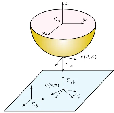
Consider a rolling robot composed of a spherical shell (carrier) actuated by internal rotors. It is assumed that the rotors have the same mass distribution and the center of mass of the system is located at the geometric center. The rotors are mounted symmetrically along orthogonal axes, as shown in Fig. 1. On each axis, the two diametrically opposite rotors are actuated in tandem. This scheme, with actuation along two orthogonal axes, was first proposed in [2] and later on studied in [8], [15].
Define the following coordinate frames (see Fig. 2):Σb is a base (inertial) frame fixed in the contact plane andΣo is a frame fixed at the geometric center of the spherical object. In addition, we introduce
Fig. 1. Rolling system with orthogonal placement of rotors.
Fig. 2. Basic frames and contact coordinates.
two contact frames, one on the objectΣc o and one on the planeΣc b. The contact coordinates are given by the anglesϑandϕ, describing the contact point on the sphere, by the displacementsxandy, describing the contact point on the plane, and by the contact angleψ, which is defined as the angle between thex-axis ofΣc o andΣc b(thez-axes of these frames are aligned, as depicted in Fig. 2). It is assumed that the frameΣc b is parallel toΣb, and in the zero configuration the axes of Σoare parallel to those ofΣb.
The position of the contact point on the sphere is parameterized asc(ϑ, ϕ) = [−Rsinϑcosϕ, Rsinϕ,−Rcosϑcosϕ]T,whereRis the radius of the sphere. In this parameterization, the origin is placed at the south pole of the sphere. In terms of the contact coordinates, the orientation matrix of the sphere (the orientation ofΣo relative toΣb) is defined asR(ψ, ϕ, ϑ) =RT
z(ψ)RTx(ϕ)RTy(ϑ)
△
= [n1 |n2 |n3], whereRx(ϕ),Ry(ϑ), andRz(ψ)are the matrices of elementary ro-tations, and the columns of the orientation matrix are defined as
n1 = ⎡
⎢ ⎣
cosϑcosψ+ sinϑsinϕsinψ
−cosϑsinψ+ sinϑsinϕcosψ
cosϑcosϕ
⎤
⎥
⎦ (1)
n2 = ⎡
⎢ ⎣
cosϕsinψ
cosϕcosψ
−sinϕ
⎤
⎥
n3= defined in projections onto the axes ofΣb. The evolution of the contact coordinates can be established from the Montana equations [16] and represented as
Note that the no-spinning constraintωz = 0, featuring the pure rolling mode, is not imposed here.
The dynamic equations for the system under consideration are de-veloped in [15]. Under the assumption that the motion does not start impulsively, the dynamic model admits the following integral
J ω+Jr
reflecting the conservation of the total angular momentum of the system about the contact point, which can be interpreted as the driving principle of the robot under consideration. Here,qiis the angle of rotation around the axisni, Jris the inertia moment of the single rotor around its axis of rotation, andJ=diag{Jx x, Jx x, Jz z}is the inertia tensor of the composite system (rolling carrier and the rotors) with respect to the contact point.Jx x =Jz z+M R2, Jz z = 23moR2 + 2Jp+Jr, where Mis the total mass of the system,mois the mass of the spherical shell, andJpis the inertia moment of the rotor about the plane orthogonal to the axis of rotation.
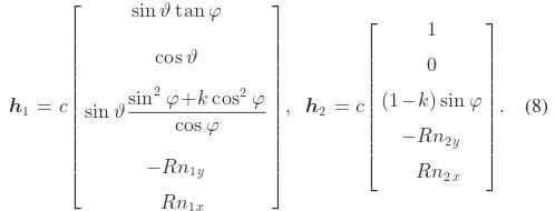
By combining (4) and (6), one obtains the following five states–two inputs driftless affine control system
˙
x=H(x) ˙q=h1(x) ˙q1+h2(x) ˙q2 (7) where the rates of the rotors angles are considered as the control inputs, and the columns of the matrixH=−JrAJ−1[n1 |n2]are defined
The motion planning problem we address in this paper consists of finding a trajectoryx(t), t∈[0, T], given the start statex(0) =xsand the final statex(T) =xf. It should be noted that for the robot under consideration, this problem cannot be solved exclusively at the level of kinematics1, by dealing only with the system (4) and finding the appropriate vector of the angular velocityω(t). The reason is that the components of the vectorωare dynamically (or, better said, inertially) constrained by the condition n3 ·J ω= 0, which follows from (6). The physical meaning of this condition is that the angular momentum of the rolling carrier must lie in in the plane through the axes of the actuated rotors.
By checking the Lie algebra rank condition, one can find [15] that the distribution formed by the vector fieldsh1,h2,h3 = [h1,h2],h4 = [h1,h3],h5 = [h2,h3], where[·,·]stands for the Lie brackets of two vector fields, has full rank unlessϑ=±π/2, i.e., the contact point lies on the great circle in the equatorial plane of the rotors axes (red line in Fig. 1). However, the distribution formed byh1,h2,h3,h4,h6, where h6 = [h1,h4], has full rank atϑ=±π/2and, therefore, the system (7) is controllable.
The existence of the singular line contrasts the robot under consider-ation to the ball–plate system. Mathematically, when the contact point gets into the singular line the degree of nonholonomy of the system (7) changes from three to four. Note that whenϑ=±π/2, the vec-torωis always on the line through the vectorn3 and the condition of dynamic realizability,n3·J ω= 0, is not satisfied. The physical meaning of this singularity line, defined byϑ=±π/2, is evident—it is impossible to generate the rolling motion of the robot along this line when the rotors axes are placed in the equatorial plane.
While the system (7) is controllable, it can be shown that it is not nilpotent, not differentially flat, and cannot be represented in chained form. The lack of special structure places it into the general class of driftless nonholonomic systems and stipulates the use of general steering techniques. To facilitate motion planning, one can devise a motion strategy composed of maneuvers for which the construction of movements is relatively easier than that conducted in the general formulation.
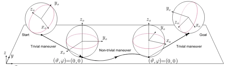
In this paper, we fabricate a motion planning strategy consisting of two trivial and one nontrivial maneuver, as depicted in Fig. 3. The trivial maneuvers are executed right before and right after the nontrivial one. In the first trivial maneuver, the contact coordinatesϑandϕare nullified, while in the second one, they are brought from zeros to desired values. Thus, in the nontrivial maneuver, the motion planning problem is solved under the assumption that at the start and end configurations, the initial and final values ofϑ and ϕare zero. The change of the contact coordinatesx, y, andψcorresponding to the trivial maneuvers can be computed in advance, and the corresponding initial and desired values for the nontrivial maneuver can be easily established.
On the whole, this general reconfiguration strategy is comparable with those considered in [9], [11]–[13] for the kinematic ball–plate system. Apart from the structural simplicity, the reason the strategy is divided into trivial and nontrivial maneuvers has also to do with the singularity lineϑ=±π/2. This line is passed only during the trivial maneuvers where the singularity does not create any computational problems. Thus, during the nontrivial maneuver, the contact point on the sphere does not leave either lower or upper hemisphere. The details of the trivial maneuver are described in the Appendix, and from now on, we concentrate on the nontrivial maneuver.
Fig. 3. Motion planning strategy.
A computational algorithm, solving the motion planning problem for the nontrivial maneuver, can be constructed with the use of the nilpotent approximation2 of the nonnilpotent system dynamics. The idea was first proposed in [20] and later developed in [17], [21]. Since the control problem for the nilpotent system can be solved exactly, the control inputs found for the nilpotent system can be used for iterative steering of the original nonnilpotent system (7). In the remainder of this paper, we compute the nilpotent approximation, construct an iterative steering algorithm, and verify it under simulation.
A. Nilpotent Approximation
Before approximating the original system (7), it is reasonable to convert it to strictly triangular form. This can be done with the use of the following input transformation
whereu1andu2are the new control inputs. This results in the following representation
˙
x=G(x)u=g1(x)u1 +g2(x)u2 (12) where the columns of the matrixGare defined as
g1 =
The nilpotent approximation of the system (12) in the neighborhood of some pointx0is obtained as follows [17], [22]. First, one transforms the original coordinatesxto local coordinatesy at the pointx0 as follows: integer such that dimLr(x
0) = 5. The weightwiof the coordinatesxi is defined by settingwj=sifns−1 < j≤ns, withns=ns(x0)and
n0= 0. Note thatrdefines the degree of nonholonomy, and the vec-tor(n1(x0), . . . , nr(x0))is the growth vector of the nonholonomic system (12).
2The conventional tangent linearization cannot be used for our purpose be-cause it does not retain the controllability property.
Having defined the local coordinatesy, one then transforms them to privileged coordinatesz. In the component form, the transformation is represented as theses is the Lie derivative of orderj−1
i= 1αi along the vector fields g1,g2, . . . ,gj−1evaluated at the pointx0.
Having constructed the transformation (15), one expresses the sys-tem (12) in the privileged coordinates and expands it in Taylor series at the origin. Finally, the nilpotent approximation of system (12) is ob-tained by collecting in the Taylor series the terms of weighted degree −1. The approximate system
˙
z= ˜G(z)u= ˜g1(z)u1+ ˜g2(z)u2 (17) is nilpotent, controllable, composed of polynomial functions, and has the same degree of nonholonomy and the same growth vector as the original system [17], [22].
In our implementation of the nontrivial maneuver, we need to con-struct the nilpotent approximation only at the south pole of the sphere whereϑ0 =ϕ0 = 0. When the point the approximation is constructed at is set asx0 = [0,0, ψ0, x0, y0]the calculations are simplified con-siderably. In particular, the matrixΓtakes the following form
Γ= [g1(x0), g2(x0), g3(x0), g4(x0), g5(x0) ]−1
In addition, whenϑ0 =ϕ0 = 0the second term of (15) vanishes and the privileged coordinateszi coincides withyi. Therefore, the trans-formation from the original to the privileged coordinates is obtained as The original system (12), (13), expressed in the privileged coordinates with the use of (21), (25), becomes
˙
By expanding this system in Taylor series at the origin and retaining the terms of weighted degree−1, one obtains the representation (17) with the vector fieldsg˜1 and˜g2defined as
The resulting approximate system is polynomial and in triangular form. The latter property facilitates the integration of the approximate dynam-ics in closed form under some well-defined control inputs.
It should be finally noted that if one setsk= 0in (31), the approx-imate system (17) will coincide with that constructed in [17] for the kinematic model of a ball–plate system with no-spinning constraint ωz = 0. However, in our model, such a setting can be only purely hypothetical because by definition (9) the inertia ratiok >1.
B. Iterative Steering
Having constructed the nilpotent approximation (17), one can use it for the iterative steering of the original system (12) from the initial xs to a desired statexf. The general idea of this approach can be formulated as follows [17].
1) Seti= 0, ti= 0, andxi =xs.
2) Setti+ 1 =ti+ ∆T, where∆Tis the movement time allocated for one iteration. Define the subgoal xd
i =xi+η(xf −xi), whereη∈[0,1]is a sufficiently small number. Compute from
(15) the image of the subgoal in the privileged coordinates,zd i, and construct a controller that steers the approximate nilpo-tent system (17) from the origin to zd
i in the time interval t∈[ti, ti+ 1]. This control problem can be solved exactly, and the control law found for the nilpotent system is then applied to the original system (12).
3) If the statex(ti+ 1)the system is brought to by the control action is far fromxf, seti=i+ 1andxi=x(ti+ 1)and repeat the iterative process.
The particular structure of the control law to steer a nilpotent sys-tem can be constructed in a variety of ways [20], [23]–[25]. In this paper, we build it in the spirit of the geometric phase approach [9], [12] because it results to simple calculations and has a clear geometric interpretation. Compared with steering the robot under consideration by sinusoids at integrally related frequencies [26], it results in well-structured trajectories and requires less iterations to reach the goal state. As in [17], the nontrivial maneuver in our construction is divided into two parts corresponding to attaining, respectively, the desired ori-entation and translation. More specifically, reconfiguring the initial statexs = [0,0, ψs, xs, ys]to the final onexf = [0,0, ψf, xf, yf]is described as follows.
First Part: In the first part, we steerϑ, ϕ, andψto the desired values 0,0, andψf regardless of the values ofxandy. The computational procedure can be summarized as follows.
1) Seti= 0, ti = 0,xi Define the control law by
u1(t) =ricosσiωt (33) u2(t) =risinσiωt (34) wheret∈[ti, ti+ 1]andσi=sign(ψf −ψi). Geometrically, in the space of the contact coordinatesϑandϕ, this control law traces a circle of radiusriin the direction defined byσi
ϑ(t) = ri
Therefore, by the end of the iteration, the contact coordinatesϑ andϕremain unchanged.
By direct integration of the approximate system (17) and (31) with the control (33) and (34), it can be shown that
z1(ti+ 1) =z2(ti+ 1) = 0, z3(ti+ 1) =σiπr2i/ω2. (37) The free parameterriis defined from the conditionz3(ti+ 1) = Ψd
i, which results in
ri=ω #
|Ψd
i|/π. (38) Thus, the control law defined by (33) and (34) steers the privi-leged coordinatesz1, z2, andz3from the origin to, respectively, 0,0, andΨd
i. By checking the first three equations of the system (12), (13), one can see that in the original coordinates, we have ϑ(ti+ 1) =ϕ(ti+ 1) = 0, butψ(ti+ 1)does not necessarily reach
3) Setxi=xi+ 1, increase the counteri=i+ 1, and repeat the calculations untilψ(ti+ 1)reaches a given vicinity ofψf. It should be noted that, since the control law (33) and (34) defines a circle in the space ofϑandϕ, one has|ϑ(t)| ≤ri/ωand|ϕ(t)| ≤ri/ω. To guarantee that the contact point does not leave the lower hemisphere, one must have
ri ω =
-η|ψf −ψi| (2k−1)π ≤
. η
2k−1 < π/2 (39) which gives the following estimate
η <(2k−1)π2/4. (40) Thus, since the inertia ratiok >1, for anyη∈[0,1]the control law (33), (34) keeps the contact point away from the singularity lineϑ= ±π/2.
1) Second Part: In the second part of the maneuver, we steerx, y to the desired valuesxf, yf without changing (in the final configura-tion) ϑ=ϕ= 0and ψ=ψf. The computational procedure can be summarized as follows.
1) Seti= 0, ti= 0,xi= [0,0, ψf,x¯s,y¯s], where¯xs,y¯s are the coordinates of the contact point in the plane attained by the end of the first part of the maneuver.
2) Setti+ 1 =ti+ 2∆T. Define the subgoal in the contact plane xd
i =xi+η(xf −xi) and yid=yi+η(yf −yi), where η∈ [0,1], and compute by (24) and (25) the image of the subgoal in the privileged coordinates
Xid = η
R(1−3k){sinψf(xf−xi) + cosψf(yf−yi)}
(41) Yd
i = η
R(1−3k){cosψf(xf−xi)−sinψf(yf−yi)}.
(42) Letω= 2π/∆T. Define the control law by
u1(t) =ricos (θi+ωt) (43) u2(t) =risin (θi+ωt) (44) fort∈[2(i−1)∆T,(2i−1)∆T]and
u1(t) =ricos (θi−ωt) (45) u2(t) =risin (θi−ωt) (46) fort∈[(2i−1)∆T,2i∆T]. Geometrically, this control law de-fines two symmetric circles in the space of the contact coordinates ϑandϕ
ϑ(t) =ri
ω {sin(θ+ωt)−sinθ} (47) ϕ(t) =ri
ω {cosθ−sin(θ+ωt)} (48) fort∈[2(i−1)∆T,(2i−1)∆T]and
ϑ(t) =ri
ω {sinθ−sin(θ+ωt)} (49) ϕ(t) =ri
ω {sin(θ+ωt)−cosθ} (50) fort∈[(2i−1)∆T,2i∆T]. Therefore, the contact variablesϑ and ϕare zero at t=ti+ (2i−1)∆T, and t=ti+ 2i∆T.
Next, since one circle is traced in clockwise direction and the other in the counterclockwise direction, by the end of the itera-tion, the angleψremains unchanged.
By direct integration of the approximate system (17), (31) with the control (43), (44) and (45), (46), it can be shown that
z1(ti+ 1) =z2(ti+ 1) =z3(ti+ 1) = 0 (51)
z4(ti+ 1) = 2πri3sin (ψf −θi)/ω3 (52) z5(ti+ 1) = 2πr3i cos (ψf −θi)/ω3. (53) The free parametersri andθi are defined from the conditions z4(ti+ 1) =Xidandz5(ti+ 1) =Yid, which results in
ri =ω
6
. (Xd
i)2+ (Yid)2
4π2 (54)
θi =ψf −arctan (Xid/Yid). (55) Thus, the control law defined by (43) and (44), as well as (45) and (46), steers the state variables of the approximate nilpotent system (17) from the origin to, respectively,[0,0,0, Xd
i, Yid]. By the geometric construction, for the original state variables, we haveϑ(ti+ 1) =ϕ(ti+ 1) = 0, andψ(ti+ 1) =ψf, butx(ti+ 1) andy(ti+ 1)do not necessarily reachxdi andydi.
3) Setxi =xi+ 1, increase the counteri=i+ 1, and repeat the calculations until the coordinates of the contact point in the plane [x(ti+ 1), y(ti+ 1)reach a given vicinity of[xf, yf].
Under the control law (43) and (44), as well as (45) and (46), the contact point in the space of the contact coordinatesϑandϕis always on the circle of radiusri/ω, with|ϑ(t)| ≤ri/ωand|ϕ(t)| ≤ri/ω. To ensure that the contact point does not leave the lower hemisphere, one needs to have
ri ω =
6
. (Xd
i)2+ (Yid)2 4π2 <
π
2. (56) By transforming this inequality with the use of (41), (42), one obtains the following estimate
η R <
π4(3k−1) 32
(xf −xi)2+ (yf −yi)2
. (57)
Thus, ifηis selected in accordance with (57), the trajectory of the contact point on the sphere is kept below the singularity lineϑ=±π/2.
Two comments are in order.
1) For the brevity of presentation, in the iterative scheme described in this section, the parameterηis a constant that must be tuned to ensure the convergence of the iterative process. A globally convergent iterative scheme with automatic adjustment ofηat every iteration is reported in [27], [28]. In principle, the pre-sented scheme can be easily adjusted to the settings of [27], [28] without modification of the control laws. Note, however, that the convergence rate for the schemes with constant and nonconstant ηcan be different.
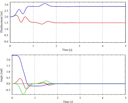
Fig. 4. Time histories ofx(red line),y(blue line) (top),ψ(blue line),ϑ(red line), andϕ(green line) (bottom) during the first part of the maneuver.
C. Simulation
The performance and effectiveness of the motion planning algorithm are tested under simulation for the nontrivial maneuver. Here, we drive the system from the initial state x0 ={0,0,3π/4,2.0,2.0} to the final statexf ={0,0,0,0,0}. In the simulation, we setR= 1,∆T = 1, k= 2.5, andη= 0.6. The units of all the dimensional quantities are specified in the SI system.
In the first part of the maneuver, where we driveψto zero regardless of the attainedxandy, we setη= 0.6. Time histories of all the state variables are shown in Fig. 4. After five iterations the error between the current and target values ofψbecomes less than 0.001, whileϑ andϕkeep zero values at the end of each iteration (integer moments of time). By the end of the first part of the maneuver, the values ofx andychange, respectively, from 2.0 to 1.51 and from 2.0 to 2.85.
In the second part of the maneuver, wherexand yare driven to the origin, we setη= 0.6. Time histories of the state variables are shown in Fig. 5. After ten iterations the error between the current and target position of the contact point on the plane, defined by the Euclidean distance
(x(t)−xf)2+ (y(t)−yf)2, becomes less than 0.001, whileϑ, ϕ, andψkeep zero values at the end of each iteration (integer moments of time).
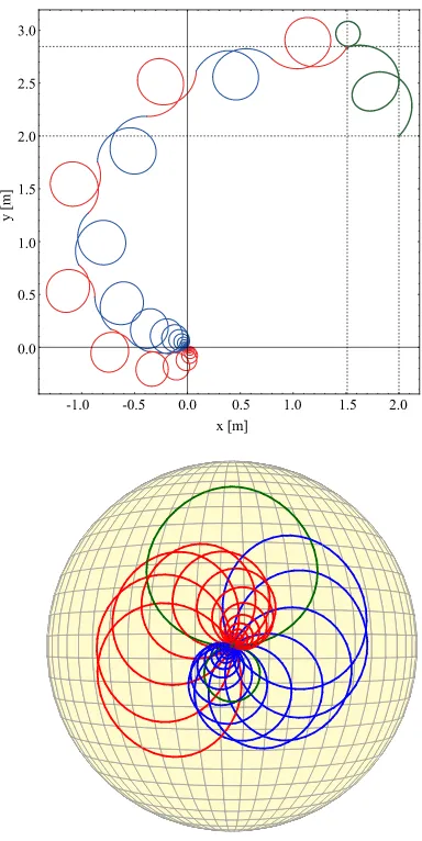
The evolution of the contact point trajectory on the sphere and on the plane is shown in Fig. 6. Here, each iteration in the first part of the maneuver is shown in green color. For the second part of the maneuver, the first half of each iteration, corresponding to the control action (43), (44), is shown in red color while the second half, corresponding to (45) and (46), is shown in blue color. As can be seen from this figure3, the magnitude of the change of the state variables is gradually decreasing as the robot approaches the target state.
While the results presented demonstrate the computational feasibil-ity of the proposed motion planning strategy, it would be also interesting to analyze the performance of the steering algorithm when the inertia parameterkof the mathematical model is changed. Although a de-tailed theoretical analysis is beyond the scope of this paper, we provide some simulation results illustrating this issue. The main problem here
3The animation of the simulation results, provided in supplementary down-loadable files, are available at http://ieeexplore.ieee.org.
Fig. 5. Time histories ofx(red line),y(blue line) (top),ψ(red line),ϑ(blue line), andϕ(green line) (bottom) during the second part of the maneuver.
is the selection of the parameterηwhich defines the convergence and the number of iterations to reach the goal state. In this connection, it should be noted that the estimates (40), (57) provide the guidance for not crossing the singularity line but have no relation to the convergence of the algorithm.
Let us revisit the simulation example considered before and change the inertia coefficient from k= 2.5 to k= 10. It is found under simulation trials that to preserve the convergence of the steering al-gorithm, one needs to decrease the parameterηfrom 0.6 to 0.5. The simulation results, presenting the evolution of the contact point trajec-tory on the sphere and on the plane, are shown in Fig. 7. Note that the magnitude of the control inputs is directly proportional to the parameter η. Therefore, the decrease ofηresults to smaller circles traced in the contact coordinatesϑandϕ, which in turn leads to the increase in the number of iterations necessary to reach the goal state.
The number of iterations as a function of η for different values of the inertia rationkcan be estimated under simulation runs. For the example considered in this section, the simulation results, including the hypothetical case ofk= 0, which corresponds to the kinematic model of pure rolling, are shown in Fig. 8. As can be seen from this figure, the interval ofηon which the iterative steering algorithm converges is gradually decreasing with the increase of the inertia ratiok. This means that the accuracy of the nilpotent approximation at a neighborhood of the south pole of the sphere is decreasing with the increase ofk.
Fig. 6. Trajectory of the contact point on the plane (top) and on the sphere (bottom) during the nontrivial maneuver fork= 2.5. The first part of the maneuver is shown in green color, while the second part is shown in red [as resulted from (43) and (44)] and blue [as resulted from (45) and (46)] colors.
(31) remains controllable but the matrixΓin (18) becomes singular. Thus, the transformation from the original to privileged coordinates tends to singularity with the increase ofk. Note also that from the physical point of view, roughly speaking, the dynamic coefficientk becomes larger with the increase of the ratio of the inertia of the spherical shell to that of the rotors. Therefore, it is realistic that driving a heavier spherical shell with lighter rotors would result in the control inputs of smaller magnitude.
It should be noted that in our algorithm, constructed in the settings of [17],ηis constant for every iteration. The iterative algorithm [27], [28] with automatic adjustment ofηconverges for any value ofk. In our numerical experiments, not reported in this paper because of the page limitation4, the latter algorithm often converges faster than the former one but not always because the actual convergence rate depends also on the initial and final configurations. Still, the pattern of the decrease of the convergence rate with the increase ofkcan be witnessed also in the globally convergent algorithm [27], [28].
4However,Mathematicasoftware scripts, implementing the algorithms with constant and nonconstantη, are available from the authors upon request.
Fig. 7. Trajectory of the contact point on the plane (top) and on the sphere (bottom) during the nontrivial maneuver fork= 10. The first part of the ma-neuver is shown in green color, while the second part is shown in red [as resulted from (43) and (44)] and blue [as resulted from (45) and (46)] colors.
Fig. 8. Number of iterations in the second part of the nontrivial maneuver as a function ofηfor different values of the inertia ratiok.
IV. CONCLUSION
Fig. 9. Trivial maneuver.
the robot, represented by a driftless control system, contains a physical singularity corresponding to the motion of the contact point along the equatorial line in the plane of the two rotors. To solve the state-to-state transfer problem, a motion planning strategy composed of two trivial and one nontrivial maneuver has been proposed. The trivial maneuvers implement motion along the geodesic line perpendicular to the singu-larity line. The nontrivial maneuver is based on an iterative steering algorithm and employs the nilpotent approximation of the originally nonnilpotent robot dynamics. The feasibility of the motion planning strategy has been verified under simulation.
In future research, apart from the experimental verification of the motion planning strategy, it would be interesting to try out different, more systematic techniques to pass through the singularity line. Theo-retical approaches to steering nonholonomic systems with singularities are reported in [22], [28]. In principle, these approaches are applicable to the rolling robot with two rotors. However, the practical construction of computationally feasible algorithms based on these approaches is not trivial and requires a special investigation.
APPENDIX
Here, we consider the trivial maneuver executed in the third step5of the motion strategy and show how to modify thex, y, andψcomponents of the vectorx0 so that rolling along a geodesic line on the sphere will guarantee arrival at the given target configurationxf. The vectorx0is then set as the target configuration for the nontrivial maneuver executed in the second step of the motion strategy.
Letϑf andϕf be the corresponding components of the vectorxf. The geodesic line connectingϑf and ϕf with the origin is defined uniquely and is perpendicular to the singularity lineϑ=±π/2. Let β+π/2be the angle of orientation of the great circle, formed by this geodesic line, with respect to the frameΣo as shown in Fig. 9. When the sphere rolls along the geodesic line it rotates around the unit vector nswhose components in the frameΣoare[cosβ,sinβ,0]T.
5The calculations in the first step are similar and can be conducted straight-forwardly in much the same way.
Letαbe the angle of rotation around the unit vectorns. The matrix of rotation aroundnscan be defined by the Rodriguez formula
Rs=I+ sinαΩ(ns) + (1−cosα)Ω2(ns) (58) whereΩ(·)is the skew-symmetric matrix used for the matrix repre-sentation of the vector product (Ω(a)b=△a×b), which gives
Rs= ⎡
⎢ ⎣
1−sin2β(1−cosα) 1
2sin 2β(1−cosα) sinβsinα 1
2 sin 2β(1−cosα) 1−cos
2β(1−cosα)−cosβsinα
sinβsinα cosβsinα cosα
⎤
⎥ ⎦.
(59) The orientation of the sphere at the final configuration can be repre-sented as
R(ψ0,0,0)Rs(β, α) =R(ψf, ϑf, ϕf) (60) where the orientation matrix of the sphereR(ψ, ϑ, ϕ) is defined in Section II. By solving this equation with respect to the unknown angles α, β, andψ0, one obtains
α= arccos (cosϑf cosϕf) (61)
β= arctan
cosϕf sinϑf sinϕf
(62)
ψ0 =β−arctan
sinϑf cosψf−cosϑfsinϕf sinψf sinϑf sinψf+cosϑf sinϕfcosψf
. (63)
Having defined the anglesα, βandψ0, one finally obtains
x0 =xf −R αcos (β−ψ0) (64)
y0 =yf −R αsin (β−ψ0). (65) It remains to be shown that the motion along the selected geodesic line is dynamically realizable. Whenαis changed as a function of time the orientation matrix of the sphereRis defined by the left hand side of (60). Therefore,
n3= [sinα(t) sin (β−ψ0),−sinα(t) cos (β−ψ0),cosα(t)]T. (66) ComputingωfromΩ(ω) = ˙RRT yields
ω=Rα˙(t)[cos (β−ψ0),sin (β−ψ0),0]T. (67) Since the last component ofωis zero, the motion is pure rolling and the contact point on the plane moves along the straight line6 connecting (x0, y0) with (xf, yf). Since J =diag{Jx x, Jx x, Jz z}, it is easily verified thatn3 ·J ω= 0, and, therefore, the motion is dynamically realizable. The velocities of the rotors, realizing this motion, are defined from (6) and obtained as
˙
q1(t) =−(n1·J ω)/Jr =−(Jx x/Jr) ˙α(t) cosβ (68) ˙
q2(t) =−(n2·J ω)/Jr =−(Jx x/Jr) ˙α(t) sinβ. (69)
REFERENCES
[1] A. Bicchi, A. Balluchi, D. Prattichizzo, and A. Gorelli, “Introducing the “Sphericle”: An experimental testbed for research and teaching in non-holonomy,” inProc. IEEE Int. Conf. Robot. Autom., Albuquerque, NM, USA, 1997, vol. 3, pp. 2620–2625.
[2] S. Bhattacharya and S. Agrawal, “Spherical rolling robot: A design and motion planning studies,”IEEE Trans. Robot. Autom., vol. 16, no. 6, pp. 835–839, Dec. 2000.
[3] A. Javadi and P. Mojabi, “Introducing glory: A novel strategy for an om-nidirectional spherical rolling robot,”ASME J. Dyn. Syst., Meas., Contr., vol. 126, no. 3, pp. 678–683, 2004.
[4] R. Balasubramanian, A. Rizzi, and M. Mason, “Legless locomotion: A novel locomotion technique for legged robots,”Int. J. Robot. Res., vol. 27, no. 5, pp. 575–594, 2008.
[5] M. Ishikawa, Y. Kobayashi, R. Kitayoshi, and T. Sugie, “The surface walker: A hemispherical mobile robot with rolling contact constraints,” inProc. IEEE/RSJ Int. Conf. Intell. Robots Syst., St. Louis, MO, USA, 2009, pp. 2446–2451.
[6] V. Joshi, R. Banavar, and R. Hippalgaonkar, “Design and analysis of a spherical mobile robot,”Mech. Mach. Theory, vol. 45, no. 2, pp. 130–136, 2010.
[7] A. Borisov, A. Kilin, and I. Mamaev, “How to control Chaplygin’s sphere using rotors: Part II,”Regular Chaotic Dyn., vol. 18, no. 1–2, pp. 144–158, 2013.
[8] V. Joshi and R. Banavar, “Motion analysis of a spherical mobile robot,” Robotica, vol. 27, no. 3, pp. 343–353, 2009.
[9] Z. Li and J. Canny, “Motion of two rigid bodies with rolling constraint,” IEEE Trans. Robot. Autom., vol. 6, no. 1, pp. 62–72, Feb. 1990. [10] V. Jurdjevic, “The geometry of the plate-ball problem,”Arch. Rational
Mech. Anal., vol. 124, no. 4, pp. 305–328, 1993.
[11] A. Marigo and A. Bicchi, “Rolling bodies with regular surface: Control-lability theory and applications,”IEEE Trans. Autom. Control, vol. 45, no. 9, pp. 1586–1599, Sep. 2000.
[12] R. Mukherjee, M. Minor, and J. Pukrushpan, “Motion planning for a spherical mobile robot: Revisiting the classical ball-plate problem,”ASME J. Dyn. Syst., Meas. Contr., vol. 124, no. 4, pp. 502–511, 2002. [13] M. Svinin and S. Hosoe, “Motion planning algorithms for a rolling sphere
with limited contact area,”IEEE Trans. Robot., vol. 24, no. 3, pp. 612–625, Jun. 2008.
[14] F. Alouges, Y. Chitour, and R. Long, “A motion-planning algorithm for the rolling-body problem,”IEEE Trans. Robot., vol. 26, no. 5, pp. 827–836, Oct. 2010.
[15] M. Svinin, A. Morinaga, and M. Yamamoto, “On the dynamic model and motion planning for a spherical rolling robot actuated by orthogonal internal rotors,”Regular Chaotic Dyn., vol. 18, no. 1–2, pp. 126–143, 2013.
[16] R. Murray, Z. Li, and S. Sastry,A Mathematical Introduction to Robotic Manipulation. Boca Raton, FL, USA: CRC, 1994.
[17] G. Oriolo and M. Vendittelli, “A framework for the stabilization of general nonholonomic systems with an application to the plate-ball mechanism,” IEEE Trans. Robot., vol. 21, no. 2, pp. 162–175, Apr. 2005.
[18] H. Hermes, “Nilpotent and high-order approximations of vector field sys-tems,”SIAM Rev., vol. 33, no. 2, pp. 238–264, 1991.
[19] A. Bella¨ıche, “The tangent space in sub-riemannian geometry,” in Sub-Riemannian Geometry, A. Bella¨ıche and J.-J. Risler, Eds. Cambridge, MA, USA: Birkh¨auser, 1996, pp. 1–78.
[20] G. Lafferriere and H. Sussmann, “A differential geometric approach to motion planning,” inNonholonomic Motion Planning, Z. Li and J. Canny, Eds. Norwell, MA, USA: Kluwer, 1993, pp. 235–270.
[21] E. Sachkova, “Approximate solution of a control problem on the basis of the nilpotent approximation,”Different. Equat., vol. 45, no. 9, pp. 1386– 1364, 2009.
[22] M. Vendittelli, G. Oriolo, F. Jean, and J.-P. Laumond, “Nonhomoge-neous nilpotent approximations for nonholonomic systems with singu-larities,”IEEE Trans. Automat. Contr., vol. 49, no. 2, pp. 261–266, Feb. 2004.
[23] R. Murray and S. Sastry, “Nonholonomic motion planning: Steering using sinusoids,”IEEE Trans. Autom. Control, vol. 38, no. 5, pp. 700–716, May 1993.
[24] S. Agrawal and S. Bhattacharya, “Optimal control of driftless nilpoten systems: Some new results,” inProc. IEEE/RSJ Int. Conf. Intell. Robots Syst., Kyongju, Korea, 1999, vol. 1, pp. 356–361.
[25] E. Sachkova, “Solution of a control problem for a nilpotent system,” Different. Equat., vol. 44, no. 12, pp. 1768–1772, 2008.
[26] A. Morinaga, M. Svinin, and M. Yamamoto, “On the motion planning problem for a spherical rolling robot driven by two rotors,” inProc. IEEE/SICE Int. Symp. Syst. Integrat., Fukuoka, Japan, 2012, pp. 704– 709.
[27] F. Jean, G. Oriolo, and M. Vendittelli, “A global convergent steering algorithm for regular nonholonomic systems,” inProc. IEEE Int. Conf. Decis. Control, Seville, Spain, 2005, pp. 7514–7519.
[28] Y. Chitour, F. Jean, and R. Long, “A global steering method for non-holonomic systems,” J. Different. Equat., vol. 254, pp. 1903–1956, 2013.
[29] B. Siciliano, L. Sciavicco, L. Villani, and G. Oriolo,Robotics: Modelling, Planning and Control, (ser. Advanced Textbooks in Control and Signal Processing). London, U.K.: Springer-Verlag, 2009.
A Selective Retraction-Based RRT Planner for Various Environments
Junghwan Lee, OSung Kwon, Liangjun Zhang, and Sung-Eui Yoon
Abstract—We present a novel randomized path planner for rigid robots to efficiently handle various environments that have different character-istics. We first present abridge line testthat can identify narrow passage regions and then selectively performs an optimization-based retraction only at those regions. We also propose anoncolliding line test, which is a dual operator to the bridge line test, as a culling method to avoid generating samples near wide-open free spaces. These two line tests are performed with a small computational overhead. We have tested our method with different benchmarks that have varying amounts of narrow passages. Our method achieves up to several times improvements over prior RRT-based planners and consistently shows the best performance across all the tested benchmarks.
Index Terms—Motion and path planning, sampling-based motion plan-ning, various environments.
I. INTRODUCTION
Robot motion planning involves computing collision-free paths for a robot and has many applications, such as part disassembly simulation, tolerance verification, protein folding, and computer graphics [1], [2]. The motion planning has been actively studied since the 1970s to develop a complete solution.
Sampling-based motion planning algorithms have been designed and successfully used to compute a probabilistic complete solution for a variety of environments. Two of the most successful algorithms include the Probabilistic Roadmap Method (PRM) [3] and Rapidly-exploring Random Tree (RRT) [4]. At a high level, as we randomly generate more samples, these techniques provide collision-free paths by capturing a larger portion of the connectivity of the free space.
One of the most challenging cases for sampling-based techniques is to efficiently handle narrow passages. In many practical motion plan-ning applications, a robot often needs to pass through narrow passages
Manuscript received November 22, 2013; accepted February 28, 2014. Date of publication May 12, 2014; date of current version August 4, 2014. This paper was recommended for publication by Associate Editor M. Vendittelli and Editor D. Fox upon evaluation of the reviewers’ comments. This work was supported in part by NRF-2013R1A1A2058052, DAPA/ADD (UD110006MD), MEST/NRF (2013-067321), and the IT R&D program of MOTIE/KEIT [10044970].
J. Lee, O. Kwon, and S.-E. Yoon are with the Department of Computer Science, Korea Advanced Institute of Science and Technology, Daejeon, Korea (e-mail: [email protected]; [email protected]; [email protected]).
L. Zhang is with Samsung Research America, San Jose, CA 95134 USA (e-mail: [email protected]).
Color versions of one or more of the figures in this paper are available online at http://ieeexplore.ieee.org.
Digital Object Identifier 10.1109/TRO.2014.2309836 1552-3098 © 2014 IEEE. Personal use is permitted, but republication/redistribution requires IEEE permission.