Chapter 02.03 Differentiation of Discrete Functions

02.03.1

Chapter 02.03

Differentiation of Discrete Functions

After reading this chapter, you should be able to:

1. find approximate values of the first derivative of functions that are given at discrete data points, and

2. use Lagrange polynomial interpolation to find derivatives of discrete functions.

To find the derivatives of functions that are given at discrete points, several methods are available. Although these methods are mainly used when the data is spaced unequally, they can be used for data that is spaced equally as well.

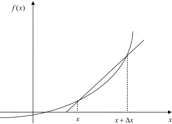
Forward Difference Approximation of the First Derivative

We know

 



  

x x f x x f x

f

x 

   



 lim0

For a finite x,

 



  

x x f x x f x f

Figure 1 Graphical representation of forward difference approximation of first derivative.

So given n1 data points



x₀,y₀

 

, x₁,y₁

 

, x₂,y₂

 

,, x_n,y_n



, the value of f(x) for

1

 

 _i

i x x

x , i0,...,n1, is given by

 

   

i i

i i

i

x x

x f x f x f

  



 

1 1

Example 1

The upward velocity of a rocket is given as a function of time in Table 1.

Table 1 Velocity as a function of time.

(s)

t v(t) (m/s)

0 0 10 227.04 15 362.78 20 517.35 22.5 602.97

30 901.67

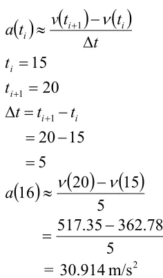
Using forward divided difference, find the acceleration of the rocket at t16 s.

Solution

To find the acceleration at t16 s, we need to choose the two values of velocity closest to s

16



t , that also bracket t16 s to evaluate it. The two points are t15 s and t20 s )

(x f

x

x

     

t

t t

v t

a i i

i _

  1 

15t_i 

20t_i1 

5

15 20

1

  

  t t_i t_i

 

   

5 15 20

16  

a

5

78 . 362 35 . 517 



= 30.914m/s2

Direct Fit Polynomials

In this method, given n1 data points



x₀,y₀

 

, x₁,y₁

 

, x₂,y₂

 

,, x_n,y_n



, one can fit a _nth

order polynomial given by

 

n

n n n

n x a a x a x a x

P  ₀  ₁  _1 1 

To find the first derivative,

 





2 1

1 2

1 2 1

)

( _{ }

  

  

 

 n

n n

n n

n a a x n a x na x

dx x dP x

P 

Similarly, other derivatives can also be found.

Example 2

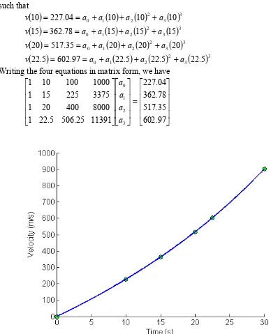
The upward velocity of a rocket is given as a function of time in Table 2.

Table 2 Velocity as a function of time. (s)

t v(t) (m/s) 0 0 10 227.04 15 362.78 20 517.35 22.5 602.97

30 901.67

Using a third order polynomial interpolant for velocity, find the acceleration of the rocket at s

16



t .

Solution

For the third order polynomial (also called cubic interpolation), we choose the velocity given by

 

3

3 2 2 1

0 at a t a t

a t

Since we want to find the velocity at t16s, and we are using a third order polynomial, we

Writing the four equations in matrix form, we have



Solving the above four equations gives 3810a₀ 4.

289 . 21

1 

a

13065 . 0

2 

a

0054606a₃ 0. Hence

 

3

3 2 2 1

0 at a t a t

a t

v    

4.381021.289t0.13065t2 0.0054606t3, 10t22.5 The acceleration at t16 is given by

 

16 

 

_16 t t v dt

d a

Given that

 

4.381021.289 0.13065 20.0054606 3, 10 22.5

t t

t t

t

v ,

 

v

 

t dt

d t a 



2 3



0054606 .

0 13065 . 0 289 . 21 3810 . 4

t t t

dt

d _{   }



21.2890.26130 0.016382 2, 10 22.5

t t

t

 

 

 

2

16 016382 .

0 16 26130 . 0 289 . 21

16   

a

29.664m/s2

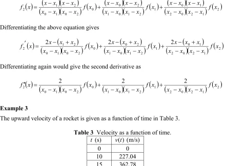
Lagrange Polynomial

In this method, given



x₀,y₀



,,



x_n,y_n



, one can fit a nth order Lagrangian polynomial given by



  n i

i i

n x L x f x

f

0

) ( ) ( )

(

where n in f_n(x) stands for the th

n order polynomial that approximates the function )

(x f

y  and



  

  n

i j

j i j

j i

x x

x x x

L

0

) (

) (x

L_i is a weighting function that includes a product of n1 terms with terms of ji

omitted.

Then to find the first derivative, one can differentiate f_n

 

x once, and so on for other derivatives.

For example, the second order Lagrange polynomial passing through

  

_



_



_{  }

_





_



_{  }

_





_



_{  }

2

Differentiating the above equation gives

 

_



_



_{  }

_



_



_{  }

_



_



_{  }

2

Differentiating again would give the second derivative as

  



   



   



  

2

The upward velocity of a rocket is given as a function of time in Table 3.

Table 3 Velocity as a function of time.

Determine the value of the acceleration at t 16s using second order Lagrangian polynomial interpolation for velocity.

Solution

DIFFERENTIATION Topic Differentiation of Discrete Functions

Summary These are textbook notes differentiation of discrete functions Major General Engineering

Authors Autar Kaw, Luke Snyder Date December 23, 2009