Asymptotically Near-Optimal Planning With Probabilistic Roadmap Spanners

Asymptotically Near-Optimal Planning With

Probabilistic Roadmap Spanners

James D. Marble

, Member, IEEE

, and Kostas E. Bekris

, Member, IEEE

Abstract_{—Asymptotically optimal motion planners guarantee} that solutions approach optimal as more iterations are performed. A recently proposed roadmap-based method, i.e., the PRM∗

ap-proach, provides this desirable property and minimizes the com-putational cost of generating the roadmap. Even for this method, however, the roadmap can be slow to construct and quickly grows too large for storage or fast online query resolution, especially for relatively high-dimensional instances. In graph theory, there are algorithms that produce sparse subgraphs, which are known as graph spanners, that guarantee near-optimal paths. This pa-per proposes different alternatives for interleaving graph spanners with the asymptotically optimalPRM∗_{algorithm. The first}

alterna-tive follows a sequential approach, where a graph spanner algo-rithm is applied to the output roadmap ofPRM∗_{. The second one}

is an incremental method, where certain edges are not considered during the construction of the roadmap as they are not necessary for a roadmap spanner. The result in both cases is an asymptoti-callynear_{-optimal motion planning solution. Theoretical analysis} and experiments performed on typical, geometric motion planning instances show that large reductions in construction time, roadmap density, and online query resolution time can be achieved with a small sacrifice of path quality through roadmap spanners.

Index Terms_{—Motion planning, near-optimality, probabilistic} roadmaps.

I. INTRODUCTION

S

AMPLING-BASED algorithms correspond to a practi-cal framework to solve high-dimensional motion planning problems. The probabilistic roadmap method (PRM_{) [1] is an}

instance of such a method that uses an offline phase to construct a graph that represents the structure of the configuration space (C-space). This graph, which is known as a roadmap, can be queried in an online phase to quickly provide solutions.

Traditionally,PRMand many related variants [2]–[7] focused on quickly finding a feasible solution. Pursuing only this

objec-Manuscript received December 30, 2011; revised August 14, 2012; accepted December 8, 2012. Date of publication January 11, 2013; date of current version April 1, 2013. This paper was recommended for publication by Associate Editor T. Simeon and Editor D. Fox upon evaluation of the reviewers’ comments. This work was supported by the National Science Foundation under Award CNS 0932423. Any opinions and findings expressed in this paper are those of the authors and do not necessarily reflect the views of the sponsor.

J. D. Marble was with the Department of Computer Science and Engineering, University of Nevada, Reno, NV 89557 USA. He is now with Sierra Nevada Corporation, Sparks, NV 89434 USA (e-mail: midorikid@gmail.com).

K. E. Bekris was with the Department of Computer Science and Engineering, University of Nevada, Reno, NV 89557 USA. He is now with the Department of Computer Science, Rutgers University, Piscataway, NJ 08854 USA (e-mail: kostas.bekris@cs.rutgers.edu).

Color versions of one or more of the figures in this paper are available online at http://ieeexplore.ieee.org.

Digital Object Identifier 10.1109/TRO.2012.2234312

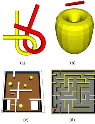
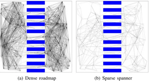
Fig. 1. (a) Roadmap constructed by an algorithm that is guaranteed to converge to optimal solution costs and (b) another roadmap constructed in such a way that guarantees convergence tonear-optimal solution costs but results in far fewer edges.

tive may result in reduced solution quality, which can be eval-uated given a variety of measures depending on the underlying task. For instance, clearance from obstacles or smoothness can be used to evaluate the quality of the solution path [8]. This study focuses on popular path quality measures that are metric func-tions, such as path length or traversal time. One standard way to improve solution quality is through path smoothing, a postpro-cessing step applied to the path returned by a planner. A more sophisticated way to improve path quality is through hybridiza-tion graphs, which combine multiple soluhybridiza-tions into a higher quality one that uses the best portions of each input path [9]. There are also algorithms that attempt to produce roadmaps, which return paths that are deformable to optimal ones after the application of smoothing [10], [11]. These smoothing-based techniques, however, can be expensive for the online resolution of a query, especially when multiple queries must be answered given the same input roadmap.

Alternatively, it is possible to construct larger, denser roadmaps that better sample the C-space by investing more preprocessing time. For instance, a planner that attempts to con-nect a new sample to every existing node in the roadmap will converge to solutions with optimal costs, a property known as asymptotic optimality. While roadmaps with this property are desirable for their high path quality, their large size can be prob-lematic. Large roadmaps impose significant costs during con-struction, storage, transmission, and online query resolution; therefore, they may not be appropriate for many applications. The recently proposedk-PRM∗ algorithm [12] minimizes the numberk of neighbors each new roadmap sample has to be tested for connection while still providing asymptotic optimal-ity guarantees. Even so, the densoptimal-ity of roadmaps produced by

k-PRM∗_{can still be high, resulting in slow online query}

resolu-tion times.

This paper argues that a viable alternative is to construct roadmaps with asymptotic near-optimality guarantees. By re-laxing the optimality requirement, it is possible to construct roadmaps that are sparser, faster to build, and can answer queries faster, while providing solution paths that are arbitrarily close to optimal. The idea is illustrated in Fig. 1.

The theoretic foundations for this study lie in graph theory. In particular, graph spanners are sparse subgraphs with guarantees on path quality. Spanner construction methods filter edges of the original graph and guarantee that any shortest path between nodes in the sparse subgraph has cost at mostt×c∗_{, wherec}∗

is the optimum path cost in the original graph, andtis an input parameter called the stretch factor. An existing method in the motion planning literature, which created roadmaps that con-tained Useful Cycles [13] was in fact producing graph spanners. In this framework, roadmap edges that pass the “usefulness” test are added to the roadmap because not doing so would violate path quality guarantees, similar to those of graph spanners. Nev-ertheless, since this method did not start from a roadmap with optimality guarantees, it did not provide any properties related to optimality.

In this study, graph spanner algorithms are combined with asymptotically optimal roadmap planners to produce planners that construct roadmap spanners. These are roadmap methods with asymptotic near-optimality guarantees. Two algorithms are proposed in this paper.

1) The first method builds a roadmap spanner in a sequential manner given an asymptotically optimal roadmap. 2) A second proposed alternative interleaves roadmap

struction with a spanner preserving filter to directly con-struct a roadmap spanner in an efficient way.

The resulting roadmaps are sparse, which is beneficial in any application where the density of the roadmap matters.

A. Related Work

Computational efficiency:There has been a plethora of tech-niques on how to sample and connect configurations so as to achieve computational efficiency in roadmap construction via a sampling-based process [2]–[6], [14]. Certain algorithms, such as the visibility-based Roadmap [4], the Incremental Map Gen-eration algorithm [6], and the Reachability Roadmap Method [15], focus on returning a connected roadmap that covers the entire configuration space. A reachability analysis of roadmap techniques suggested that connecting roadmaps is more diffi-cult than covering theC-space [7]. Furthermore, a method is available to characterize the contribution of a sample to the ex-ploration of theC-space [16], but it does not address how the connectivity between samples contributes to the resulting path quality once the space has been explored.

Path Quality:Work on creating roadmaps that contain high-quality paths has been motivated by the objective to efficiently resolve queries without the need for a postprocessing optimiza-tion step of the returned path. One technique aims to compute all different homotopic solutions [11], while Path Deforma-tion Roadmaps compute paths that are deformable to optimal ones [10]. Another approach inspired by Dijkstra’s algorithm

extracts optimal paths from roadmaps for specific queries [17] but may require very dense roadmaps. The Useful Cycles ap-proach implicitly creates a roadmap spanner with small number of edges [13] and has been combined with the Reachability Roadmap Method to construct connected roadmaps that cover 2-D and 3-D C-spaces to provide high-quality paths [18]. A method has been introduced that filters nodes from a roadmap if they do not improve path quality measures [19].

Tree-based planners and dynamics:Roadmaps cannot be con-structed for problems where there is no solution for the two-point boundary value problem, i.e., it is not easy to compute a path that connects exactly two states of a moving system. On the other hand, tree-based kinodynamic planners [20], [21] can operate on such environments. Tree-based algorithms are very effec-tive for single-query planning. They do not provide, however, the preprocessing properties of roadmaps, and they tend to be slower for multiquery applications. Regarding sparsity, a tree is already a sparse graph and it becomes disconnected when removing edges. It has been shown that theRRTalgorithm pro-duces arbitrarily bad paths with high probability and will miss high-quality paths even if they are easy to find [12], [22]. Any-timeRRT[23] has been proposed as an approach that practically improves path quality in an incremental manner. Tree-based planners for kinodynamic problems can still benefit from an approximate roadmap to estimate distances between states and the goal region that take into accountC-space obstacles. Such distance estimates can be used as a heuristic in tree expansion to bias the selection of states closer to the goal and solve problems with dynamics faster [24], [25].

Asymptotic Optimality:TheRRG_,RRT∗_{, and}PRM∗ _families

of algorithms [12] provide asymptotic optimality for general configuration spaces.RRGandRRT∗ are based onRRT, which is a tree-based planner. The anytimeRRT∗approach [26] extends

RRT∗with anytime planning in dynamic environments and can incrementally improve path quality.PRM∗is a modification of standardPRM. The proposed techniques in this paper are based onk-PRM∗, i.e., a variation ofPRM∗, which will be described in detail in Section II-A.

B. Contribution

This paper describes two methods to construct roadmap span-ners based on previous work by the authors [27], [28]. It is shown that both methods guarantee a constant factor of asymptotic op-timality, i.e., provide asymptotic near-optimality. The first alter-native is theSequential Roadmap Spanner(SRS_{) method [27],}

which has the following characteristics.

1) It constructs a sparse graph given a dense roadmap. 2) It provides asymptotic guarantees on the number of edges. 3) It provides asymptotically near-optimal solutions. 4) It has the same asymptotic time complexity asPRM.

The second alternative is theIncremental Roadmap Spanner

(IRS) method [28], which has the following characteristics. 1) It directly constructs sparse roadmaps using a sampling

and filtering process.

2) In environments where collision detection is expensive, it constructs roadmaps in a computationally efficient way. 3) It provides asymptotically near-optimal solutions. 4) It has an asymptotic time complexity close to that ofPRM.

IRS _{can incrementally construct a roadmap spanner in a}

continuous space, while most graph spanner algorithms are for-mulated to operate on an existing roadmap. BecauseIRS

em-ploys the framework of an asymptotically optimal planner, i.e.,

PRM∗ _{[12], it provides asymptotic near-optimality guarantees}

that related approaches, such as the Useful Cycles method, do not [13]. IRS _{is shown to produce significantly sparser}

roadmaps thank-PRM∗experimentally.

Both methods balance two extremes in terms of motion plan-ning solutions. On one hand, the connected component heuristic forPRMcan connect the space very quickly with a very sparse roadmap, but can produce solutions with arbitrarily high cost. On the other hand, thek-PRM∗ algorithm provides asymptot-ically optimal roadmaps that tend to be very dense and slow to construct. WithIRS, it is possible to tune the solution qual-ity degradation relative tok-PRM∗_{and select a parameter, i.e.,}

the stretch factor, that will return solutions arbitrarily close to the optimal ones while still constructing sparse roadmaps effi-ciently.

The theoretical guarantees on path quality that these tech-niques provide are tested empirically in a variety of motion planning problems in SE(2) and SE(3). Experiments show that as the desired stretch factor increases, most of the roadmap edges can be removed while increasing mean path length by a relatively small amount. Often, this increase in path length can be significantly reduced by utilizing smoothing. Path degra-dation is most pronounced for paths that are very short, while longer paths are less affected. The sparsity of the roadmaps pro-duced is a valuable feature in itself, but with IRS, a marked decrease in construction time is also measured.

Relative to the authors’ previous work [27], [28], this paper provides a more detailed description and analysis of the two proposed algorithms under a common framework for the devel-opment of roadmap spanners. Furthermore, it provides a direct comparison of the two methods using a new, common set of experiments. The experiments suggest that the incremental ap-proach is able to produce sparser roadmaps than the sequential alternative for the same stretch factor.

II. FOUNDATIONS

A robot can be abstracted as a point in a d-dimensional configuration-space (C-space) where the set of collision-free configurations is defined as Cfree ⊂C [29]. The experiments performed in this paper take place in the spaces of 2-D and 3-D rigid body transformations (SE(2)andSE(3) correspond-ingly). The proposed methods are also applicable to anyC-space that is a metric and probability space for reasons described in Section III. OnceCfreecan be calculated for a particular robot,

one needs to specify initial and goal configurations to define an instance of the path planning problem:

Definition 1 (Path Planning Problem): Given a set of collision-free configurations Cfree ⊂C, initial and goal con-figurationsqinit, qgoal∈Cfreefind a continuous curveσ∈Σ = {ρ|ρ: [0,1]→Cfree}, whereσ(0) =qinitandσ(1) =qgoal.

ThePRMalgorithm [1] can find solutions to the path planning problem by first sampling configurations inCfreeand then trying to connect them to neighboring configurations with local paths. It starts with an empty roadmap and then iterates until some stopping criterion is satisfied. For each iteration, a configuration in Cfree is sampled and a set of neighbors is identified. For each of these neighbors, an attempt is made to connect them to the sampled configuration with a local planner. If such a curve exists inCfree, i.e., it is collision free, an edge between the two configurations is added to the roadmap.

The offline phase of the algorithm is completed once some user-defined stopping criterion is met. The result is a graphG= (V, E)that reflects the connectivity ofCfree and can be used to answer query pairs of the form(qinit, qgoal)∈Cfree×Cfree, where qinit is the starting configuration, andqgoal is the goal configuration. This type of graph is known as a roadmap. The procedure for querying it is to addqinitandqgoalto the roadmap in the same way sampled configurations are added during the offline phase. Then, a discrete graph search is performed to find a path on the roadmap between the two configurations.

A. k-PRM∗

Asymptotic optimality is the property that, given enough time, solutions to the path planning problem will almost surely con-verge to the optimum, as defined by a cost function.

Definition 2 (Asymptotic Optimality in Path Planning):An algorithm isasymptotically optimal if, for any path planning problem(Cfree, qinit, qgoal)and cost functionc: Σ→R≥0with a robust optimal solution of finite cost c∗_{, the probability of}

finding a solution of costc∗ _{converges to 1 as the number of}

iterations approaches infinity.

Asymptotic optimality is defined only forrobustly feasible

problems, as defined in the presentation ofk-PRM∗_{[12]. Such}

problems have a minimum clearance around the optimal solution and cost functions with a continuity property.

The method with which neighbors are selected is an impor-tant variable in thePRM_{. Infully connected} PRM_{, all existing}

samples in the roadmap are considered neighbors, regardless of distance. This results in a highly dense roadmap. The number of edges can be reduced by restricting the maximum distance that two samples are considered neighbors, as insimplePRM. The number of edges still grows quadratically with the number of samples in this case. The density of the roadmap can be fur-ther reduced by considering only a fixed number of the nearest samples as neighbors, as ink-nearestPRM. Althoughk-nearest

PRMproduces the sparsest roadmaps of the three, it does not provide asymptotic optimality [12]. The properties of these and the following variations are described in Table I.

The PRM∗ _and k-PRM∗ _{algorithms rectify this by}

TABLE I

VARIATIONS OFPRMANDTHEIRPROPERTIES

of the current size of the roadmap. Specifically, fork-PRM∗, the number of nearest neighbors isk(n) =kPRMlogn, where

kPRM> e(1 + 1/d),nis the number of roadmap nodes, anddis the dimensionality of the space. Roadmaps that are constructed by these variations are asymptotically optimal [12]. Neverthe-less, the number of neighbors selected for connection attempts still grows with each iteration.

B. Graph Spanners

A graph spanner, as formalized in the related literature [30], is a sparse subgraph. Given a weighted graph G= (V, E), a subgraphGS = (V, ES ⊂E)is at-spanner ofGif for all pairs

of vertices(v1, v2)∈V, the shortest path betweenv1 andv2 inGS is no longer thanttimes the shortest path between v1 andv2inG. Becausetspecifies the amount of additional length allowed in the solution returned by the spanner, it is known as thestretch factorof the spanner.

A simple method for spanner construction, which is a gener-alization of Kruskal’s algorithm for the minimum spanning tree, is given in Algorithm 1 [31]. Instead of accepting only edges that connect disconnected components, this algorithm also accepts edges that add useful cycles. Kruskal’s algorithm is recovered by settingtto a large value, such that no cycle is useful enough to be added.

The inclusion criteria on line 4 ensure that no edges required to maintain the spanner property are left out. From the global ordering of the edges of line 1, it has been shown that the number of edges retained is reduced from a potentialO(n2_)to

O(n)[31].

The quadratic number of shortest path queries puts the time complexity into O(n3_{logn); however, much work has been} done to find algorithms that reduce this. Most perform clustering in a preprocessing step, and one method uses this idea to reduce the time complexity toO(m), wheremis the number of edges [32]. It is this algorithm that was chosen for the sequential approach presented in this study.

TABLE II

SPANNERALGORITHMS ANDTHEIRPROPERTIES

A number of alternatives take advantage of the implicit weights of a Euclidean metric space to improve performance. Many of these operate oncompleteEuclidean graphs [33], [34]. They cannot be easily used inC-spaces with obstacles because obstacles remove edges of the complete graph. Table II lists a range of spanner algorithms that can be applied to weighted graphs along with their properties.

III. APPROACH

The central concept proposed in this study is that of asymp-totic near-optimality. This new property is a relaxation of asymptotic optimality that permits an algorithm to converge to a solution that is withinttimes the cost of the optimum.

Definition 3 (Asymptotically Near-Optimal Path Planning):

An algorithm is asymptotically near-optimal if, for any path planning problem(Cfree, qinit, qgoal)and cost functionc: Σ→

R≥0that admit a robust optimal solution with finite costc∗, the probability that it will find a solution of costc≤tc∗ _{for some}

stretch factort≥1 converges to 1 as the number of iterations approaches infinity.

The high-level approach is to combine the construction of an asymptotically optimal roadmap with the execution of a spanner algorithm. These two tasks can be performed either sequentially (first find the roadmap and then compute the spanner), or incre-mentally by interleaving the steps of each task.

A. Sequential Roadmap Spanner

An asymptotically optimal roadmapGgenerated byk-PRM∗

can be used to construct an asymptotically near-optimal roadmap GS by selectively removing existing edges.

Apply-ing an appropriate spanner algorithm to the roadmap accom-plishes this and is referred to in this paper as theSRSalgorithm. Algorithm 2 outlines the operation of theSRSmethod at a high level. It first makes a call to thek-PRM∗algorithm, which pop-ulates the graph(V, E), and thenSRScomputes the spanner of

(V, E). A stopping criterion is assumed to be used byk-PRM∗

so that it returns in finite time.

respect to the number of edges is adopted. The graph spanner method employed bySRS_{is outlined below.}

1) Randomized(2a−1)Spanner Algorithm [32]: The in-put to this approach (see Algorithm 3) corresponds to the sets of vertices and weighted edges of the roadmap,V andE, and the spanner parameter a. The stretch factor t is a function of the input parametera:t= (2a−1). The output isES, i.e., the

edges of the spanner. There are two parts in the algorithm. First, clusters are formed. Second, the clusters are joined to each other. A clustercis a set of vertices. A clusteringKi is the set of

clusters at iterationi. Vertices only belong to one cluster in any clustering. Before the first iteration, each vertex is made into its own, singleton cluster to form the initial K0 clustering. With each successive iteration, the following steps are performed.

1) A subset of the previous iteration’s clusters is sampled randomly [see Fig. 2(b)].

2) The vertices in the remaining, unsampled clusters are then split up and added to their neighboring clusters [see Fig. 2(c)].

3) Vertices with no adjacent clusters in thecurrentclustering are connected to all adjacent clusters from theprevious

clustering [see Fig. 2(d)].

This is repeated until⌊a₂⌋iterations have been performed. In the second part of the algorithm (line 22), the clusters are joined by the shortest edge that connects them to their neighbors [see Fig. 2(e)].

Two auxiliary functions will be useful in the definition of the (2a−1) spanner algorithm. The functionE(v, c)returns all edges in the setEfrom the vertexvto vertices in clusterc. Similarly, the functionE(c, c′)returns all edges inEconnecting any vertex in clustercto any in clusterc′_.

Fig. 2. Randomized (2a−1) spanner algorithm for a= 2. (a) Initial roadmap. (b) Sample clusters. (c) Closest cluster. (d) No adjacent cluster. (e) Cluster joining. (f) Final spanner.

The clustering K0 is initialized (line 2) so that each ver-tex becomes its own cluster. Lines 5–7 randomly sample the last iteration’s clusters with probabilityn−1

a [see Fig. 2(b)]. A probability smaller than 1 has the important effect of reducing the number of clusters at each iteration. As a notational conve-nience,Virepresents the vertices that belong to sampled clusters

at iterationi(line 8).

Sampled clusters are expanded in lines 11–14. Here, the clos-est, neighboring, sampled cluster,nv, is found for each vertex

that is not a member of a sampled cluster. The algorithm shown in Algorithm 4 adds edges to the spanner that connect the new vertices to their clusters.

For those vertices that are adjacent to sampled clusters, lines 3–5 add the shortest edge to the nearest sampled cluster and discards the others. To maintain the spanner property, edges to other unsampled clusters that are shorter than this must also be retained (lines 6–12). At the conclusion of each iteration (see lines 15–20 in Algorithm 3), intracluster edges are removed fromE.

After all⌊a₂⌋iterations have completed, K⌊a

2⌋ contains the

final clusters, each of which is a tree rooted at the cluster center.

which of these must be added to the spanner. In Algorithm 5, only the shortest edge to each neighboring cluster is added. To maintain the spanner property, clusters from the previous iteration must also be considered whenais even (line 4).

In this manner, a sparse roadmap spanner can be constructed from a dense roadmap. Nevertheless, constructing an entire dense roadmap before removing edges can be wasteful. Ev-ery edge in the dense roadmap has been checked for collisions, but many of these will be discarded by the spanner algorithm. In the next section, an incremental spanner algorithm is de-scribed, which accepts or rejects edges as they are considered for addition to the roadmap and before collision checking is per-formed. It sacrifices asymptotic time complexity for a reduction in the number of collision checks, which is frequently the most expensive operation in motion planning.

B. Incremental Roadmap Spanner

TheIRS (see Algorithm 6) takes the idea of the SRSone step further. Here, roadmap and spanner construction are inter-leaved. When the roadmap algorithm adds an edge, the spanner algorithm can reject it before collision detection is performed. Before discussing the implementation of the algorithm, some

subroutines must be defined for the particular C-space being worked on:

SAMPLEFREEuniformly samples a random configuration in

Cfree.

NEAR(V, v, k)returns thekconfigurations in setV that are nearest to configurationvwith respect to a metric function. This can be implemented as a linear search through the members of

V or as something more involved, such as a nearest neighbors search in akd-tree [39].

COLLISIONFREE(v, u)detects if there is a path between con-figurations v anduin Cfree. Generally, a local planner plots a curve in C from v tou. Points along this curve are tested for membership inCfree, and if any fail, the procedure returns

false.

STOPPINGCRITERIONdetermines when to stop looking for a solution. Some potential stopping criteria are

1) a solution of sufficient quality has been found; 2) allotted time or memory have been exhausted; 3) enough of theC-space has been covered; or some combination of these or other criteria.

WEIGHT (v, u) returns the positive edge weight of (v, u). In the context of motion planning, the weight of an edge is frequently the cost of moving the robot from configurationvto configurationualong the curve provided by a local planner.

SHORTESTPATH (V, E, v, u) returns the cost of the shortest path betweenv andu. Note that the actual shortest path cost is not required, just whether it is larger thanttimes the weight of the edge (v, u). Instead of naively applying a full graph search, a length limited variation of A∗_{search can be employed.}

In this variation, the search is aborted if a node with a cost value f > t×w(v, u)is expanded. When this happens, it is known that there is no path fromvtouwith an acceptable cost. Additionally, edges that connect two disconnected components can be added without doing any kind of search because the shortest path cost in this case is infinite.

For each iteration, SAMPLEFREEis called and returnsv∈Cfree (line 3). The sampled vertex is added to the roadmap (line 4). The number of nearest neighbors is calculated (line 5). The setU

of thek-nearest neighbors ofvis found by calling NEAR(V, v, k)

(line 6). If NEARdoes not already returnU ordered by distance fromv, then it must be sorted on line 7. For each potential edge connectingvto a neighbor inU, the inclusion criteria must be met before it is added to the roadmap. First, if a path exists betweenvanduwith cost less thanttimes the weight of(v, u), then that edge can be rejected because it contributed little to path quality (line 9). Second, the edge must be checked for collision (line 10), as it is typically the case in the PRM_{framework. If}

the local planner does not succeed in finding a curve inCfree, the edge is rejected. If the edge passes both inclusion tests, it is added to the roadmap (line 11). Then, the next iteration is started.

A notable departure thatIRSmakes from Algorithm 1 is that the edges are not ordered globally. This ordering is not required to preserve solution quality, however, as will be shown later. A

localordering of potential edges is performed on line 7. This does not affect the theoretical bounds on solution quality but can be seen as a heuristic that improves the sparsity of the final roadmap.

Since the spanner property is tested before the collision check, many expensive collision checks can be avoided. This property greatly improves running time for practically sized roadmaps.

IV. ANALYSIS

The properties ofSRS_andIRS_{are formally described in this}

section.

A. Asymptotic Near-Optimality

Theorem 1:SRSis asymptotically near-optimal.

Proof:Asymptotic near-optimality (see Definition 3) differs from asymptotic optimality (see Definition 2) only in that the solution costs must converge to withinttimes the optimal cost instead of the actual optimal cost.

It is known that solutions on roadmaps produced byk-PRM∗

converge to the optimal costs [12]. A t-spanner of such a roadmap is guaranteed to have solutions within t times the cost of those in the original roadmap.SRS_{producest-spanners}

of roadmaps constructed byk-PRM∗_{. Therefore, solutions on}

roadmaps produced bySRS_{converge to withinttimes the cost of}

optimal, as the construction of the original roadmap byk-PRM∗

goes to infinity.

Theorem 2:IRSis asymptotically near-optimal.

Proof:This proof also relies on the asymptotic optimality of

k-PRM∗ on whichIRSis based. The proposed technique has two differences fromk-PRM∗.

First, on line 7, the potential neighbors of a newly added vertex are ordered by nondecreasing distance from the new vertex. This would have no effect on the asymptotic optimality ofk-PRM∗_{because edges are rejected based solely on collisions}

with obstacles. The order that edges are tested for collisions has no effect on those tests. The second difference, which is shown on line 9, adds an additional acceptance criterion. This has the

effect of making the edges in a roadmap output byIRSa subset of those output byk-PRM∗.

Consider a pair of roadmapsG= (V, E)returned byk-PRM∗

andGS = (V, ES ⊂E)returned byIRS. For each edge(v, u)

inE/ES, there was a path fromvtouwith a cost less thant

times the weight of(v, u). This invariant is enforced by line 9. The shortest pathσinGbetween any two pointsa, b∈V has costc∗_{. This path may contain edges that are inEbut not inE}

S.

For each of these edges(v, u), there exists an alternate path in

GS, with costc(v ,u)≤t·w(v, u). Therefore, there is a pathσS

betweenaandbinGS with cost(σv ,uS )c(v ,u)≤t·c∗. In other words, since each detour is no longer thanttimes the cost of the portion of the optimal path it replaces, the sum cost of all of the detours will not exceedttimes the total cost of the optimal path. This way, as construction time goes to infinity, the roadmap returned byIRSbecomes near-optimal with probability 1.

B. Time Complexity

The time complexity analysis ofSRS_andIRS_{can be}

under-stood in relation to the complexity ofk-PRM∗_{. For each of then}

iterations ofk-PRM∗_{, a nearest neighbors search and collision}

checking must be performed. Anǫ-approximate nearest neigh-bor search can be done inlogntime producing k(n) = logn

neighbors. The edge connecting the current iteration’s sample to each of these neighbors must be checked for collision at a cost of

logdptime, wherepis the number of obstacles. Therefore, the total running time ofk-PRM∗isO

n·(logn+ logn·logdp)

, which simplifies toO(n·logn·logdp).

1) Time complexity breakdown for each of n iterations of

k-PRM∗_{(ignoring constant time operations):}

a) NEAR(ǫ-approximate):logn

b) For eachlognneighbors: i) COLLISIONFREE:logdp.

The time complexity of SRS is adding to the complexity of k-PRM∗ the complexity of the graph-spanner algorithm (O(kn)). The linear complexity of the graph-spanner algorithm is dominated by that ofk-PRM∗. Thus, overall the complexity ofSRS_{isO(n·logn·log}d_p).

1) Time complexity breakdown for each of n iterations of

IRS_{(ignoring constant time operations):}

a) NEAR(ǫ-approximate):logn

b) Neighbor ordering:logn·log logn

c) For eachlognneighbors: i) COLLISIONFREE:logdp

ii) SHORTESTPATH> t·WEIGHT:td_logn·log(td

logn)(average case).

ForIRS, two additional steps are performed. At every itera-tion,k= lognneighbors must be sorted by their distance to the sampled vertex. Many implementations of NEARreturn the list of neighbors in order of distance, in which case, the cost of this operation can be zero. If this is not the case, however, the cost of sorting thesekneighbors isO(klogk), and sincek= logn, the final result isO

logn·log (logn)

.

andm=nlogn, since each node is connected to at mostlogn

neighbors. The shortest path algorithm will expand only the ver-tices with path cost fromvthat is lower thant·w(v, u). This is due to the fact that the algorithm requires only knowledge about the existence of a path betweenvandushorter than this bound. Whent= 1, the number of nodes expanded by such a search is, at most,k(n)∈O(logn). Assuming a uniform sampling dis-tribution, the expected number of nodes that may be expanded whent >1is proportional totd_{logn(based on the volume of}

ad-dimensional hyper-sphere). This brings theexpectedtime complexity ofIRS_to

O(n·(logn+ logn·log logn

+ logn·(logdp+tdlogn·log (tdlogn))))

which simplifies toO(n·logn·td_{logn·log (t}d_{logn)), or, for}

fixedtandd:

O(n·log2n·log logn)

which is asymptotically slower thank-PRM∗. However, as will be shown experimentally, the very large constants involved in collision checking, which is avoided by IRS, makes IRS a computationally efficient alternative, at least for roadmaps of practical size.

C. Size Complexity

The number of edges in a spanner produced by Algorithm 3 isO(an1+1

a)which also bounds the number of edges produced bySRS.

IRSis inspired by Algorithm 1, which producesO(n)edges (with constants related totandd). This bound does not hold for IRS _{itself. Without a global ordering of edges, there is}

no guarantee that the minimum spanning tree is contained within the spanner. Because of this, the space complexity can-not be bounded lower than that provided byk-PRM∗_{, which is}

O(nlogn). The experimental results, however, suggest that the dominant term is linear as the number of edges added at each iteration appear to converge to a constant.

V. EVALUATION

All experiments were executed using the Open Motion Plan-ning Library (OMPL) [40] on 2-GHz processors with 4 GB of memory. Four representative environments were chosen from those distributed with OMPL.

Alpha puzzle: Cfree is a subset of SE(3) and is highly constrained in this classical motion planning benchmark [see Fig. 3(a)].

Bug trap: A rod-shaped robot must orient itself to fit through the narrow passage and escape a 3-D version of the classical bug trap [SE(3); see Fig. 3(b)].

Cubicles: Two floors of loosely constraining walls and obsta-cles must be navigated [SE(3); see Fig. 3(c)].

Maze: A complex environment in a lower dimensional (SE(2)) space [see Fig. 3(d)].

For each of these environments and stretch factor combina-tion, ten roadmaps with 50 000 vertices each were generated.

Fig. 3. Environments used in the experiments with example configurations for the robot. (a) Alpha puzzle. (b) Bug trap. (c) Cubicles. (d) Maze.

On each of these roadmaps, 100 random start and goal pairs were queried over the course of construction, and various qual-ities of the resulting solutions were measured. An additional

SE(3)environment (apartment) was considered in Fig. 4 as a representative case for high collision detection costs.

A. Construction Time

Although the expected asymptotic time complexity ofIRS

is worse than that ofk-PRM∗_{, the large constants involved in}

collision detection dominate the running time in many cases. SinceIRS_{reduces the number of collision checks required at}

the cost of including a call to a graph search algorithm (due to the check on line 9), running time can be reduced for higher stretch factors. This is shown in Fig. 4, where a stretch factor oft= 2

allowsIRSto construct a 50 000-node roadmap in under two-thirds of the time ofk-PRM∗. The diminishing returns shown for higher stretch factors reflect the larger area of the graph that must be searched for shortest paths. Construction times for the other experiments are shown in Fig. 5. Whether a time savings is achieved is dependent on features of the environment that affect collision checking such as the density of the obstacles and how expensive each collision check is to perform.

B. Space Requirements

The reduction in edges by the roadmap spanners is shown in Fig. 6. While each roadmap contains the same number of ver-tices (50 000), the space required for connectivity information is reduced by up to 85%. AlthoughSRShas a lower asymptotic bound for the number of edges produced, IRS shows much better results, in practice, for the same stretch factor.

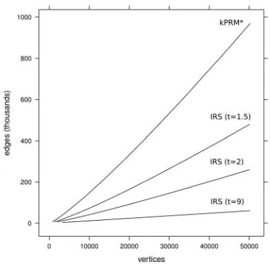
Fig. 7 shows the number of edges added to a roadmap as the number of nodes grows for both k-PRM∗ _and IRS_{. In these}

Fig. 4. Construction time and roadmap density for k-PRM∗ andIRSin the apartment environment (shown below). When the cost to perform colli-sion detection is high, as in the complex apartment environment, practically sized roadmap spanners can be constructed faster because fewer edges must be checked for collision.

Fig. 5. Mean construction times of 50 000-node roadmaps for each environ-ment. Error bars indicate the minimum and maximum times over ten runs.

Fig. 6. Mean roadmap density of ten different 50 000-node roadmaps for each environment. The minimum and maximum values are within the size of the icons.

Fig. 7. Density growth for a roadmap constructed in the alpha environment. The reduction in the number of edges increases with stretch factor and grows approximately linearly with the number of vertices.

C. Solution Quality

In Fig. 8, path quality is measured by querying a roadmap with 100 random start and goal configurations. The lengths of the resulting paths increase as the number of edges in the spanner is reduced. It is important, however, to note that for these random starting and goal configurations, the average extra cost is significantly shorter than the worst case guaranteed by the stretch factor.

The worst degradation happens for short paths, where taking a detour of even a single vertex can increase the path length by a large factor. Path quality degradation inIRS_{is plotted in}

Fig. 9 as a function of its length in a roadmap generated by

Fig. 8. Mean solution length for 100 random query pairs on ten different 50 000-node roadmaps compared with thek-PRM∗outcome. Path length in-creases when the stretch factor inin-creases. The increase is much less than the theoretical guarantee.

Fig. 9. Mean path length degradation for different stretch factors as a function of the path length in the original roadmap in the bug-trap environment with 5000 vertices. All shortest paths starting from ten random vertices in five different roadmaps were measured.

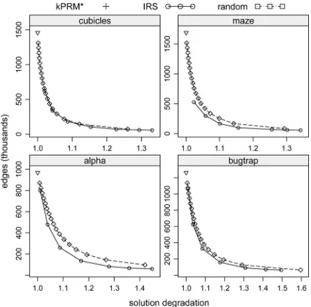
over five different roadmaps. In Figs. 10 and 11, the tradeoff between roadmap density and path quality is compared. It can be observed from these figures thatIRSdominates bothSRS

and a na¨ıve approach where random edges are removed. Table III provides the mean roadmap construction time in minutes for the algorithms in the different environments.

Overall, the results show that theSRSis not able to provide a large reduction in edges for low stretch values. For example, in one environment, it was only able to reduce the edge count by 15.3% for a stretch factor of 3. For higher stretch factors, e.g., up to 17, most of the edges (77% to 85%) can be removed bySRS_,

while increasing mean path length by a small amount (10% to

Fig. 10. Tradeoff between solution length and roadmap density averaged over 100 random query pairs on ten different 50 000-node roadmaps for each envi-ronment. Each data point forIRSandSRSrepresents a different stretch factor from 1.25 to 9. Except for the alpha environment,IRSdominatesSRSin these two performance measures.

Fig. 11. Tradeoff between solution length and roadmap density averaged over 100 random query pairs on ten different 50 000-node roadmaps for each envi-ronment. Each data point forIRSrepresents a different stretch factor from 1.25 to 9. Each data point for the “random” method represents the probability an edge being removed from 5% to 90%.IRSdominates this random method in these two performance measures.

TABLE III

Fig. 12. Mean search time for 100 random query pairs on ten different 50 000-node roadmaps for each environment. Higher stretch factors produce roadmaps with fewer edges that can be searched more quickly.

25%). TheIRS_{described in Algorithm 1 was able to achieve a}

70.5% edge reduction for relatively small stretch factors.

D. Roadmap Search Time

The time it took to perform an A∗ _{search on the resulting}

roadmap was also measured. The reported value does not include the time it takes to connect the start and goal configurations. As shown in Fig. 12, removing edges from the roadmaps reduces the query resolution time by up to 70%.

While reduced online query resolution time is presented here as a separate benefit, it is dependent on the size of the generated roadmap. Larger roadmaps generally result in longer search times. Experiments suggest that search time has an approxi-mately linear relationship with the number of edges in roadmaps of these environments. This is illustrated in Fig. 13 and explains the similarity between Figs. 6 and 12.

E. Effects of Smoothing

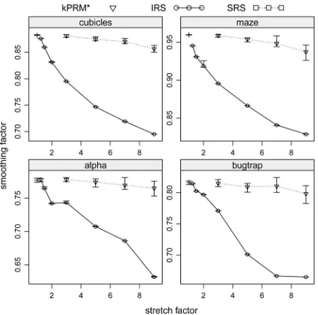
For each query, a simple approach for path smoothing was tested. Nonconsecutive vertices on the path that were near each other were tested for potential collision-free connectivity. If they could be connected, then the path is shortened by removing the intervening vertices. This is a greedy and local method for smoothing, but it can be executed very quickly and produces impressive results. In Fig. 14, the smoothing factor is reported as the ratio of the smoothed cost to the unsmoothed cost. The time taken to smooth the solutions was between 0.01 and 0.7 s. A smoothing factor of less than one indicates that there was some improvement due to smoothing. Note thatk-PRM∗ _{has yet to}

converge to the optimal solution; therefore, applying smoothing still improves the solution path. The solutions from roadmap spanners constructed with higher stretch factors showed more

Fig. 13. In these environments (and in the environment shown in Fig. 4), roadmap search time has an approximately linear relationship to the density of the roadmap.

Fig. 14. Ratio of the cost of the smoothed solution to that of the unsmoothed one for 100 random query pairs on ten different 50 000-node roadmaps for each environment.

improvement after smoothing, reducing their cost relative to the smoothedk-PRM∗_solutions.

VI. DISCUSSION

A. Selecting a Stretch Factor

metrics such as preprocessing time, roadmap size, or online search time, a higher value should be used.

If preprocessing time is not an issue, then the parameter space can be searched until the highest value fortis found that pro-duces a roadmap that fits into the space or search time allowed. Some tasks will have a natural method for optimizing the stretch factor. Define the total cost of completing a motion planning query as the time to search the roadmap (a) plus the time it takes to travel the path (b). Increasing t will decrease a, but increaseb. Decreasingtwill have the opposite affect. Then, the stretch factortcan be optimized to minimize the worst case for

a+b.

If limits on detour length relative to a known optimum can be defined, then the stretch factor can be chosen directly. For example, if a path that can be followed by a robot is twice as long as another, the robot can be prevented from taking the undesirable path by settingtto less than 2.

B. Path Quality Guarantees Versus Actual Average Path Quality

The path quality guarantees in this study are based on the worst possible situation where every edge along an optimal path has been replaced by a detour that ist-times longer. While this is possible, it has a very low probability of happening for any query that must traverse a significant portion of the roadmap. For very short paths, that will utilize fewer roadmap edges, it is more likely. Nevertheless, the fact that some edges have, necessarily, not been removed pushes the average path degradation lower than the stretch factor limit, especially for queries with longer optimal paths. A practical measure of roadmap path quality might be the average degradation over all possible paths. In general, this is difficult to predict before actually constructing a roadmap but may be possible to calculate for environments with simple cost functions and no obstacles.

C. Applicability to Problems With Arbitrary Cost Functions

In order to guarantee near-optimal solutions, the cost function used in the methods presented here must be Lipschitz continu-ous. Such a function is relatively easy to construct for kinematic systems. If no guarantees are required, then an arbitrary cost function may be employed. The practical benefits of faster con-struction and search time, smaller roadmap thank-PRM∗_{, and}

better path quality than k-PRM _{should still be present with}

most cost functions. If the cost function does not create a metric space, then a graph search algorithm other than A∗ _{should be}

used. Any work on asymptotically optimal planners that operate with arbitrary cost functions moves in an orthogonal direction and should be possible to integrate with the current work on roadmap spanners.

VII. CONCLUSION

This study has shown that it is practical to compute sparse roadmaps inC-spaces that guarantee asymptotic near-optimality. These roadmaps have considerably fewer edges than roadmaps with asymptotically optimal paths, while resulting in

small degradation in path quality relative to the asymptotically optimal ones. The stretch factor parameter provides the ability to tune this tradeoff. The experiments confirm that roadmaps with low stretch factors have high path quality but are denser.

The current approach removes only roadmapedges. It is also the case, however, that nodes of the roadmap are redundant for the computation of near-optimal paths. Consecutive work to this one is investigating how to remove nodes so that the quality of a path answering a query in the continuous space is guaranteed not to get worse than a stretch factor [41]–[43].

It is important to study the type of near-optimality guarantees that can be provided in finite time, as in practice, a stopping criterion is employed to stop sampling-based algorithms. Fur-thermore, identifying the expected path quality degradation of a roadmap spanner will be a better indication of practical per-formance. Another direction to consider is to evaluate these algorithms in higher dimensional challenges, such as planning of articulated robots. The current experiments do not trend in a way that would suggest that problems would arise and the theoretical analysis covers these challenges.

Finally, it is important to study the relationship of roadmap spanners with methods that guarantee the preservation of the homotopic path classes in theC-space [10]. Intuitively, homo-topic classes tend to be preserved by the spanner because the removal of an important homotopic class will have significant effects on the path quality.

ACKNOWLEDGMENT

The authors would like to thank the anonymous reviewers and the Associate Editor of the IEEE TRANSACTIONS ONROBOTICS

for their constructive comments and feedback.

REFERENCES

[1] L. E. Kavraki, P. Svestka, J.-C. Latombe, and M. Overmars, “Probabilistic roadmaps for path planning in high-dimensional configuration spaces,”

IEEE Trans. Robot. Autom., vol. 12, no. 4, pp. 566–580, Aug. 1996. [2] N. M. Amato, O. B. Bayazit, L. K. Dale, C. Jones, and D. Vallejo,

“OBPRM: An obstacle-based PRM for 3D workspaces,” inProc. Work-shop Algorithm. Found. Robot., 1998, pp. 155–168.

[3] L. J. Guibas, C. Holleman, and L. E. Kavraki, “A probabilistic roadmap planner for flexible objects with a workspace medial-axis-based sampling approach,” inProc. IEEE/RSJ Int. Conf. Intell. Robot. Syst., Oct. 1999, vol. 1, pp. 254–259.

[4] T. Simeon, J.-P. Laumond, and C. Nissoux, “Visibility-based probabilistic roadmaps for motion planning,”Adv. Robot. J., vol. 41, no. 6, pp. 477–494, 2000.

[5] G. Sanchez and J.-C. Latombe, “A single-query, bi-directional probabilis-tic roadmap planner with lazy collision checking,” inProc. Int. Symp. Robot. Res., 2001, pp. 403–418.

[6] D. Xie, M. Morales, R. Pearce, S. Thomas, J.-L. Lien, and N. M. Amato, “Incremental map generation (IMG),” presented at the Workshop Algo-rithm. Found. Robot., New York, Jul. 2006.

[7] R. Geraerts and M. H. Overmars, “Reachability-based analysis for proba-bilistic roadmap planners,”J. Robot. Autonom. Syst., vol. 55, pp. 824–836, 2007.

[8] R. Wein, J. van den Berg, and D. Halperin, “Planning high-quality paths and corridors amidst obstacles,”Int. J. Robot. Res., vol. 27, no. 11–12, pp. 1213–1231, Nov. 2008.

[10] L. Jaillet and T. Sim´eon, “Path deformation roadmaps: Compact graphs with useful cycles for motion planning,”Int. J. Robot. Res., vol. 27, nos. 11/12, pp. 1175–1188, 2008.

[11] E. Schmitzberger, J. L. Bouchet, M. Dufaut, D. Wolf, and R. Husson, “Capture of homotopy classes with probabilistic roadmap,” in Proc. IEEE/RSJ Int. Conf. Intell. Robot. Syst., 2002, vol. 3, Lausanne, Switzer-land, pp. 2317–2322.

[12] S. Karaman and E. Frazzoli, “Sampling-based algorithms for optimal motion planning,”Int. J. Robot. Res., vol. 30, no. 7, pp. 846–894, Jun. 2011.

[13] D. Nieuwenhuisen and M. H. Overmars, “Using cycles in probabilistic roadmap graphs,” inProc. IEEE Int. Conf. Robot. Autom., Apr./May 2004, vol. 1, pp. 446–452.

[14] E. Plaku, K. E. Bekris, B. Y. Chen, A. M. Ladd, and L. E. Kavraki, “Sampling-based roadmap of trees for parallel motion planning,”IEEE Trans. Robot. Autom., vol. 21, no. 4, pp. 587–608, Aug. 2005.

[15] R. Geraerts and M. H. Overmars, “Creating small graphs for solving mo-tion planning problems,” inProc. IEEE Int. Conf. Meth. Models Autom. Robot., 2005, pp. 531–536.

[16] M. A. Morales, R. Pearce, and N. M. Amato, “Metrics for analyzing the evolution of C-space models,” inProc. IEEE Int. Conf. Robot. Autom., May 2006, pp. 1268–1273.

[17] J. Kim, R. A. Pearce, and N. M. Amato, “Extracting optimal paths from roadmaps for motion planning,” inProc. IEEE Int. Conf. Robot. Autom., vol. 2, Taipei, Taiwan, Sep. 14–19, 2003, pp. 2424–2429.

[18] R. Geraerts and M. H. Overmars, “Creating high-quality roadmaps for motion planning in virtual environments,” inProc. IEEE/RSJ Int. Conf. Intell. Robot. Syst., Beijing, China, Oct. 2006, pp. 4355–4361.

[19] R. Pearce, M. Morales, and N. Amato, “Structural improvement filtering strategy for PRM,” presented at the Robot. Sci. Syst., Zurich, Switzerland, Jun. 2008.

[20] D. Hsu, R. Kindel, J. C. Latombe, and S. Rock, “Randomized kinodynamic motion planning with moving obstacles,”Int. J. Robot. Res., vol. 21, no. 3, pp. 233–255, Mar. 2002.

[21] S. M. LaValle and J. J. Kuffner, “Randomized kinodynamic planning,”

Int. J. Robot. Res., vol. 20, no. 5, pp. 378–400, May 2001.

[22] O. Nechushtan, B. Raveh, and D. Halperin, “Sampling-diagrams au-tomata: A tool for analyzing path quality in tree planners,” presented at the Workshop Algorithm. Found. Robot., Singapore, Dec. 2010. [23] D. Ferguson and A. Stentz, “Anytime RRTs,” inProc. IEEE/RSJ Int. Conf.

Intell. Robot. Syst., Beijing, China, Oct. 2006, pp. 5369–5375.

[24] K. Bekris and L. Kavraki, “Informed and probabilistically complete search for motion planning under differential constraints,” presented at the 1st Int. Symp. Search Tech. Artif. Intell. Robot., Chicago, IL, Jul. 2008. [25] Y. Li and K. E. Bekris, “Learning approximate cost-to-go metrics to

im-prove sampling-based motion planning,” presented at the IEEE Int. Conf. Robot. Autom., Shanghai, China, May 9–13, 2011.

[26] S. Karaman, M. Walter, A. Perez, E. Frazzoli, and S. Teller, “Anytime motion planning using the RRT∗_{,” presented at the IEEE Int. Conf. Robot.} Autom., Shanghai, China, May 2011.

[27] J. D. Marble and K. E. Bekris, “Computing spanners of asympotically op-timal probabilistic roadmaps,” inProc. IEEE/RSJ Int. Conf. Intell. Robot. Syst., San Francisco, CA, Sep. 2011, pp. 4292–4298.

[28] J. D. Marble and K. E. Bekris, “Asymptotically near-optimal is good enough for motion planning,” presented at the Symp. Robot. Res., Flagstaff, AZ, Aug. 2011.

[29] T. Lozano-Perez, “Spatial planning: A configuration space approach,”

IEEE Trans. Comput., vol. C-32, no. 2, pp. 108–120, Feb. 1983. [30] D. Peleg and A. Sch¨affer, “Graph spanners,”J. Graph Theor., vol. 13,

no. 1, pp. 99–116, 1989.

[31] I. Alth¨ofer, G. Das, D. Dobkin, D. Joseph, and J. Soares, “On sparse spanners of weighted graphs,”Discr. Comput. Geometr., vol. 9, no. 1, pp. 81–100, 1993.

[32] S. Baswana and S. Sen, “A Simple and linear time randomized algo-rithm for computing sparse spanners in weighted graphs,”Random Struct. Algorithm., vol. 30, no. 4, pp. 532–563, Jul. 2007.

[33] J. M. Keil, “Approximating the complete Euclidean graph,” inProc. 1st Scandinav. Workshop Algorithm Theor.. London, U.K.: Springer-Verlag, 1988, pp. 208–213.

[34] J. Gao, L. J. Guibas, and A. Nguyen, “Deformable spanners and applica-tions,”Comput. Geometr. Theor. Appl., vol. 35, nos. 1/2, pp. 2–19, Aug. 2006.

[35] E. Cohen, “Fast algorithms for constructing t-spanners and paths with stretch t,”SIAM J. Comput., vol. 28, no. 1, pp. 210–236, 1998.

[36] B. Awerbuch, B. Berger, L. Cowen, and D. Peleg, “Near-linear time con-struction of sparse neighborhood covers,”SIAM J. Comput., vol. 28, no. 1, pp. 263–277, 1998.

[37] L. Roditty, M. Thorup, and U. Zwick, “Deterministic constructions of approximate distance oracles and spanners,” inProc. Int. Colloq. Autom. Lang. Programm., 2005, pp. 261–272.

[38] M. Thorup and U. Zwick, “Approximate distance oracles,”J. Assoc. Com-put. Mach., vol. 52, no. 1, pp. 1–24, Jan. 2005.

[39] J. L. Bentley, “Multidimensional binary search trees used for associative searching,”Commun. Assoc. Comput. Mach., vol. 18, no. 9, pp. 509–517, Sep. 1975.

[40] I. A. S¸ucan, M. Moll, and L. E. Kavraki. (2013). The open mo-tion planning library. IEEE Robot. Autom. Mag. [Online]. Available: http://ompl.kavrakilab.org

[41] J. D. Marble and K. E. Bekris, “Towards small asymptotically near-optimal roadmaps,” presented at the IEEE Int. Conf. Robot. Autom., St. Paul, MN, May 14–18, 2012.

[42] A. Dobson, A. Krontiris, and K. E. Bekris, “Sparse roadmap spanners,” presented at the Workshop Algorithm. Found. Robot., Cambridge, MA, Jun. 13–15, 2012.

[43] A. Dobson and K. E. Bekris, “Sparse roadmaps spanners for asymptot-ically near-optimal motion planning,” Int. J. Robot. Res., 2013, to be published.

James D. Marble(M’12) received the Bachelor’s and Master’s degrees in computer science and engi-neering from the University of Nevada, Reno, where he worked with Dr. K. Bekris on motion planning.

Specifically, his work has focused on near-optimal sampling-based algorithms. Toward this goal, he has contributed in the development of the PRACSYS open-source software platform for motion planning, replanning, and multirobot coordination. Since the summer of 2012, he has been with the Sierra Nevada Corporation, Sparks, NV, as a Software Engineer.

Kostas E. Bekris (M’07) received the Bachelor’s degree in computer science from the University of Crete, Crete, Greece, in 2001 and the Master’s and Doctoral degrees in computer science from Rice Uni-versity, Houston, TX, in 2004 and 2008, respectively, where he worked with Prof. L. Kavraki.

Until June 2012, he served as an Assistant Pro-fessor with the Department of Computer Science and Engineering, University of Nevada, Reno. Since July 2012, he has been with the Department of Computer Science, Rutgers University, as an Assistant Profes-sor. He is heading the PRACSYS group (http://www.pracsylab.org), which is part of the Computational Biomedicine, Modeling, and Imaging Center. His research interests include optimal motion planning, planning for systems with challenging dynamics, as well as multirobot planning and applications in robotics, cyber-physical systems, simulations, and games. His research lab has been supported by the National Science Foundation, the Office of Naval Re-search, and the National Aeronautics and Space Administration.