Petroleum Prodcution Engineering free download for u

• ISBN: 0750682701

Preface

The advances in the digital computing technology in the last decade have revolutionized the petroleum industry. Using the modern computer technologies, today’s petro-leum production engineers work much more efficiently than ever before in their daily activities, including analyz-ing and optimizanalyz-ing the performance of their existanalyz-ing pro-duction systems and designing new propro-duction systems. During several years of teaching the production engineer-ing courses in academia and in the industry, the authors realized that there is a need for a textbook that reflects the current practice of what the modern production engineers do. Currently available books fail to provide adequate information about how the engineering principles are ap-plied to solving petroleum production engineering prob-lems with modern computer technologies. These facts motivated the authors to write this new book.

This book is written primarily for production engineers and college students of senior level as well as graduate level. It is not authors’ intention to simply duplicate gen-eral information that can be found from other books. This book gathers authors’ experiences gained through years of teaching courses of petroleum production engineering in universities and in the petroleum industry. The mission of the book is to provide production engineers a handy guide-line to designing, analyzing, and optimizing petroleum production systems. The original manuscript of this book has been used as a textbook for college students of under-graduate and under-graduate levels in Petroleum Engineering.

This book was intended to cover the full scope of pe-troleum production engineering. Following the sequence of oil and gas production process, this book presents its contents in eighteen chapters covered in four parts.

Part I contains eight chapters covering petroleum pro-duction engineering fundamentals as the first course for the entry-level production engineers and undergraduate students. Chapter 1 presents an introduction to the petro-leum production system. Chapter 2 documents properties of oil and natural gases that are essential for designing and analysing oil and gas production systems. Chapters 3 through 6 cover in detail the performance of oil and gas wells. Chapter 7 presents techniques used to forecast well production for economics analysis. Chapter 8 describes empirical models for production decline analysis.

Part II includes three chapters presenting principles and rules of designing and selecting the main components of petroleum production systems. These chapters are also written for entry-level production engineers and under-graduate students. Chapter 9 addresses tubing design. Chapter 10 presents rule of thumbs for selecting com-ponents in separation and dehydration systems. Chapter 11 details principles of selecting liquid pumps, gas com-pressors, and pipelines for oil and gas transportation.

Part III consists of three chapters introducing artificial lift methods as the second course for the entry-level pro-duction engineers and undergraduate students. Chapter 12 presents an introduction to the sucker rod pumping system and its design procedure. Chapter 13 describes briefly gas lift method. Chapter 14 provides an over view of other artificial lift methods and design procedures.

Part IV is composed of four chapters addressing pro-duction enhancement techniques. They are designed for production engineers with some experience and graduate

students. Chapter 15 describes how to identify well prob-lems. Chapter 16 deals with designing acidizing jobs. Chapter 17 provides a guideline to hydraulic fracturing and job evaluation techniques. Chapter 18 presents some relevant information on production optimisation tech-niques.

Since the substance of this book is virtually boundless in depth, knowing what to omit was the greatest difficulty with its editing. The authors believe that it requires many books to describe the foundation of knowledge in petro-leum production engineering. To counter any deficiency that might arise from the limitations of space, the book provides a reference list of books and papers at the end of each chapter so that readers should experience little diffi-culty in pursuing each topic beyond the presented scope.

Regarding presentation, this book focuses on presen-ting and illustrapresen-ting engineering principles used for designing and analyzing petroleum production systems rather than in-depth theories. Derivation of mathematical models is beyond the scope of this book, except for some special topics. Applications of the principles are illustrated by solving example problems. While the solutions to some simple problems not involving iterative procedures are demonstrated with stepwise calculations, compli-cated problems are solved with computer spreadsheet programs. The programs can be downloaded from the publisher’s website (http://books.elsevier.com/companions/ 9780750682701). The combination of the book and the computer programs provides a perfect tool kit to petrol-eum production engineers for performing their daily work in a most efficient manner. All the computer programs were written in spreadsheet form in MS Excel that is available in most computer platforms in the petroleum industry. These spreadsheets are accurate and very easy to use. Although the U.S. field units are used in the com-panion book, options of using U.S. field units and SI units are provided in the spreadsheet programs.

This book is based on numerous documents including reports and papers accumulated through years of work in the University of Louisiana at Lafayette and the New Mexico Institute of Mining and Technology. The authors are grateful to the universities for permissions of publish-ing the materials. Special thanks go to the Chevron and American Petroleum Institute (API) for providing Chev-ron Professorship and API Professorship in Petroleum Engineering throughout editing of this book. Our thanks are due to Mr. Kai Sun of Baker Oil Tools, who made a thorough review and editing of this book. The authors also thank Malone Mitchell III of Riata Energy for he and his company’s continued support of our efforts to develop new petroleum engineering text and professional books for the continuing education and training of the industry’s vital engineers. On the basis of the collective experiences of authors and reviewer, we expect this book to be of value to the production engineers in the petrol-eum industry.

List of Symbols

A area, ft2

Ab total effective bellows area, in:2

Aeng net cross-sectional area of engine piston, in:2 Afb total firebox surface area, ft2

A0_i inner area of tubing sleeve, in:2 A0

o outer area of tubing sleeve, in:2

Ap valve seat area, gross plunger cross-sectional area, or inner area of packer, in:2

Apump net cross-sectional area of pump piston, in:2 Ar cross-sectional area of rods, in:2

At tubing inner cross-sectional area, in:2 o_{API API gravity of stock tank oil}

B formation volume factor of fluid, rb/stb b constant 1:5105_{in SI units}

Bo formation volume factor of oil, rb/stb Bw formation volume factor of water, rb/bbl CA drainage area shape factor

Ca weight fraction of acid in the acid solution Cc choke flow coefficient

CD choke discharge coefficient

Cg correction factor for gas-specific gravity Ci productivity coefficient of laterali Cl clearance, fraction

Cm mineral content, volume fraction Cs structure unbalance, lbs

Ct correction factor for operating temperature ct total compressibility, psi1

Cp specific heat of gas at constant pressure, lbf-ft/lbm-R

C

Cp specific heat under constant pressure evaluated at cooler

Cwi water content of inlet gas, lbmH2O=MMscf

D outer diameter, in., or depth, ft, or non-Darcy flow coefficient, d/Mscf, or molecular diffusion coefficient, m2_=s

d diameter, in.

d1 upstream pipe diameter, in.

d2 choke diameter, in.

db barrel inside diameter, in. Dci inner diameter of casing, in. df fractal dimension constant 1.6 Dh hydraulic diameter, in. DH hydraulic diameter, ft Di inner diameter of tubing, in. Do outer diameter, in.

dp plunger outside diameter, in. Dpump minimum pump depth, ft Dr length of rod string, ft

E rotor/stator eccentricity, in., or Young’s modulus, psi

Ev volumetric efficiency, fraction ev correction factor

ep efficiency Fb axial load, lbf

FCD fracture conductivity, dimensionless FF fanning friction factor

Fgs modified Foss and Gaul slippage factor fhi flow performance function of the vertical

section of laterali

fLi inflow performance function of the horizontal section of laterali

fM Darcy-Wiesbach (Moody) friction factor Fpump pump friction-induced pressure loss, psia

fRi flow performance function of the curvic section of laterali

fsl slug factor, 0.5 to 0.6 G shear modulus, psia

g gravitational acceleration, 32:17 ft=s2

Gb pressure gradient below the pump, psi/ft gc unit conversion factor, 32:17 lbmft=lbfs2

Gfd design unloading gradient, psi/ft Gi initial gas-in-place, scf

Gp cumulative gas production, scf G1

p cumulative gas production per stb of oil at the beginning of the interval, scf

Gs static (dead liquid) gradient, psi/ft G2 mass flux at downstream, lbm=ft2=sec

GLRfm formation oil GLR, scf/stb GLRinj injection GLR, scf/stb

GLRmin minimum required GLR for plunger lift, scf/ bbl

GLRopt,o optimum GLR at operating flow rate, scf/stb GOR producing gas-oil ratio, scf/stb

GWR glycol to water ratio, gal TEG=lbmH2O

H depth to the average fluid level in the annulus, ft, or dimensionless head

h reservoir thickness, ft, or pumping head, ft hf fracture height, ft

HP required input power, hp

HpMM required theoretical compression power, hp/ MMcfd

Ht total heat load on reboiler, Btu/h Dh depth increment, ft

DHpm mechanical power losses, hp

r_hi pressure gradient in the vertical section of laterali, psi/ft

J productivity of fractured well, stb/d-psi Ji productivity index of laterali.

Jo productivity of non-fractured well, stb/d-psi K empirical factor, or characteristic length for

gas flow in tubing, ft

k permeability of undamaged formation, md, or specific heat ratio

kf fracture permeability, md

kH the average horizontal permeability, md kh the average horizontal permeability, md ki liquid/vapor equilibrium ratio of compoundi kp a constant

kro the relative permeability to oil kV vertical permeability, md

L length, ft , or tubing inner capacity, ft/bbl Lg length of gas distribution line, mile LN net lift, ft

Lp length of plunger, in.

M total mass associated with 1 stb of oil M2 mass flow rate at down stream, lbm/sec

MWa molecular weight of acid MWm molecular weight of mineral

N pump speed, spm, or rotary speed, rpm n number of layers, or polytropic exponent for

gas

NAc acid capillary number, dimensionless NCmax maximum number of cycles per day nG number of lb-mole of gas

nL number of mole of fluid in the liquid phase Nmax maximum pump speed, spm

np number of pitches of stator N1

p cumulative oil production per stb of oil in place at the beginning of the interval Nf

p,n forcasted annual cumulative production of fractured well for yearn

Nnf

p,n predicted annual cumulative production of nonfractured well for yearn

Nno

p,n predicted annual cumulative production of non-optimized well for yearn

Nop

p,n forcasted annual cumulative production of optimized system for yearn

NRe Reunolds number

Ns number of compression stages required Nst number of separation stages1

nV number of mole of fluid in the vapor phase Nw number of wells

DNp,n predicted annual incremental cumulative production for yearn

P pressure, lb=ft2 p pressure, psia pb base pressure, psia

pbd formation breakdown pressure, psia Pc casing pressure, psig

pc critical pressure, psia, or required casing pressure, psia, or the collapse pressure with no axial load, psia

pcc the collapse pressure corrected for axial load, psia

Pcd2 design injection pressure at valve 2, psig

PCmin required minimum casing pressure, psia pc,s casing pressure at surface, psia pc,v casing pressure at valve depth, psia Pd pressure in the dome, psig pd final discharge pressure, psia peng,d engine discharge pressure, psia peng,i pressure at engine inlet, psia

pf frictional pressure loss in the power fluid injection tubing, psi

Ph hydraulic power, hp

ph hydrostatic pressure of the power fluid at pump depth, psia

phf wellhead flowing pressure, psia

phfi flowing pressure at the top of laterali, psia pL pressure at the inlet of gas distribution line,

psia

pi initial reservoir pressure, psia, or pressure in tubing, psia, or pressure at stagei, psia pkd1 kick-off pressure opposite the first valve, psia

pkfi flowing pressure at the kick-out-point of laterali, psia

pL pressure at the inlet of the gas distribution line, psia

Plf flowing liquid gradient, psi/bbl slug Plh hydrostatic liquid gradient, psi/bbl slug pLmax maximum line pressure, psia

po pressure in the annulus, psia

pout output pressure of the compression station, psia

Pp Wp=At, psia pp pore pressure, psi

ppc pseudocritical pressure, psia ppump,i pump intake pressure, psia ppump,d pump discharge pressure, psia Pr pitch length of rotor, ft pr pseudoreduced pressure

Ps pitch length of stator, ft, or shaft power, ftlbf=sec

ps surface operating pressure, psia, or suction pressure, psia, or stock-tank pressure, psia psc standard pressure, 14.7 psia

psh slug hydrostatic pressure, psia psi surface injection pressure, psia psuction suction pressure of pump, psia Pt tubing pressure, psia

ptf flowing tubing head pressure, psig pup pressure upstream the choke, psia Pvc valve closing pressure, psig Pvo valve opening pressure, psig pwh upstream (wellhead) pressure, psia pwf flowing bottom hole pressure, psia

pwfi the average flowing bottom-lateral pressure in laterali, psia

pwfo dynamic bottom hole pressure because of cross-flow between, psia

pc

wf critical bottom hole pressure maintained during the production decline, psia pup upstream pressure at choke, psia P1 pressure at point 1 or inlet, lbf=ft2

P2 pressure at point 2 or outlet, lbf=ft2

p1 upstream/inlet/suction pressure, psia

p2 downstream/outlet/discharge pressure, psia

p

p average reservoir pressure, psia

p

pf reservoir pressure in a future time, psia

p

p0 average reservoir pressure at decline time

zero, psia

p

pt average reservoir pressure at decline timet, psia

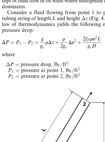
DP pressure drop, lbf=ft2

Dp pressure increment, psi

dp head rating developed into an elementary cavity, psi

Dpf frictional pressure drop, psia Dph hydrostatic pressure drop, psia

Dpi avg the average pressure change in the tubing, psi D_{po avg} the average pressure change in the annulus,

psi

D_psf safety pressure margin, 200 to 500 psi Dpv pressure differential across the operating

valve (orifice), psi Q volumetric flow rate q volumetric flow rate Qc pump displacement, bbl/day qeng flow rate of power fluid, bbl/day QG gas production rate, Mscf/day qG glycol circulation rate, gal/hr qg gas production rate, scf/d

qg,inj the lift gas injection rate (scf/day) available to the well

qgM gas flow rate, Mscf/d

qg,total total output gas flow rate of the compression station, scf/day

qh injection rate per unit thickness of formation, m3_=sec-m

qi flow rate from/into layeri, or pumping rate, bpm

qi,max maximum injection rate, bbl/min qL liquid capacity, bbl/day Qo oil production rate, bbl/day qo oil production rate, bbl/d

qpump flow rate of the produced fluid in the pump, bbl/day

Qs leak rate, bbl/day, or solid production rate, ft3_=day

qs gas capacity of contactor for standard gas (0.7 specific gravity) at standard temperature (1008F), MMscfd, or sand production rate, ft3_=day

qsc gas flow rate, Mscf/d

qst gas capacity at standard conditions, MMscfd qtotal total liquid flow rate, bbl/day

qwh flow rate at wellhead, stb/day R producing gas-liquid ratio, Mcf/bbl, or

dimensionless nozzle area, or area ratio Ap=Ab, or the radius of fracture, ft, or gas constant, 10:73 ft3_{-psia=lbmol-R}

r distance between the mass center of counterweights and the crank shaft, ft or cylinder compression ratio

ra radius of acid treatment, ft Rc radius of hole curvature, in. re drainage radius, ft reH radius of drainage area, ft Rp pressure ratio

Rs solution gas oil ratio, scf/stb rw radius of wellbore, ft

rwh desired radius of wormhole penetration, m

R2 _A

o=Ai

r_Ri vertical pressure gradient in the curvic section of laterali, psi/ft

S skin factor, or choke size,1⁄64 in.

SA axial stress at any point in the tubing string, psi

Sf specific gravity of fluid in tubing, water¼1, or safety factor

Sg specific gravity of gas, air¼1

So specific gravity of produced oil, fresh water¼1 Ss specific gravity of produced solid, fresh

water¼1

St equivalent pressure caused by spring tension, psig

Sw specific gravity of produced water, fresh water¼1

T temperature,8R

t temperature,8F, or time, hour, or retention time, min

Tav average temperature,8R Tavg average temperature in tubing,8F Tb base temperature,8R, or boiling point,8R Tc critical temperature,8R

Tci critical temperature of componenti,8R Td temperature at valve depth,8R TF1 maximum upstroke torque factor

TF2 maximum downstroke torque factor

Tm mechanical resistant torque, lbf-ft

tr retention time5:0 min Tsc standard temperature, 5208R Tup upstream temperature,8R Tv viscosity resistant torque, lbf-ft

T1 suction temperature of the gas,8R

T

T average temperature,8R u fluid velocity, ft/s um mixture velocity, ft/s

uSL superficial velocity of liquid phase, ft/s uSG superficial velocity of gas phase, ft/s V volume of the pipe segment, ft3

v superficial gas velocity based on total cross-sectional areaA, ft/s

Va the required minimum acid volume, ft3 Vfg plunger falling velocity in gas, ft/min Vfl plunger falling velocity in liquid, ft/min Vg required gas per cycle, Mscf

Vgas gas volume in standard condition, scf VG1 gas specific volume at upstream, ft3=lbm

VG2 gas specific volume at downstream, ft3=lbm

Vh required acid volume per unit thickness of formation, m3_=m

VL specific volume of liquid phase, ft3=mollb, or volume of liquid phase in the pipe segment, ft3_{, or liquid settling volume, bbl, or liquid}

specific volume at upstream, ft3_=lbm

Vm volume of mixture associated with 1 stb of oil, ft3_{, or volume of minerals to be removed, ft}3

V0 pump displacement, ft3

VP initial pore volume, ft3 Vr plunger rising velocity, ft/min Vres oil volume in reservoir condition, rb Vs required settling volume in separator, gal Vslug slug volume, bbl

Vst oil volume in stock tank condition, stb Vt At(DVslugL), gas volume in tubing, Mcf VVsc specific volume of vapor phase under

standard condition, scf/mol-lb

V1 inlet velocity of fluid to be compressed, ft/sec

V2 outlet velocity of compressed fluid, ft/sec

n₁ specific volume at inlet, ft3_=lb

n₂ specific volume at outlet, ft3_=lb

w fracture width, ft, or theoretical shaft work required to compress the gas, ft-lbf=lbm

Wair weight of tubing in air, lb/ft Wc total weight of counterweights, lbs Wf weight of fluid, lbs

Wfi weight of fluid inside tubing, lb/ft Wfo weight of fluid displaced by tubing, lb/ft WOR producing water-oil ratio, bbl/stb Wp plunger weight, lbf

Ws mechanical shaft work into the system, ft-lbs per lb of fluid

ww fracture width at wellbore, in.

w

w average width, in.

X volumetric dissolving power of acid solution, ft3mineral/ ft3solution

xf fracture half-length, ft

xi mole fraction of compoundiin the liquid phase

x1 free gas quality at upstream, mass fraction

ya actual pressure ratio yc critical pressure ratio

yi mole fraction of compoundiin the vapor phase

yL liquid hold up, fraction

Z gas compressibility factor in average tubing condition

z gas compressibility factor zb gas deviation factor atTbandpb

zd gas deviation factor at discharge of cylinder, or gas compressibility factor at valve depth condition

zs gas deviation factor at suction of the cylinder z1 compressibility factor at suction conditions

zz the average gas compressibility factor DZ elevation increase, ft

Greek Symbols

a Biot’s poroelastic constant, approximately 0.7 b gravimetric dissolving power of acid solution,

lbmmineral=lbmsolution

«0 _{pipe wall roughness, in.} f porosity, fraction h pump efficiency g 1.78¼ Euler’s constant ga acid specific gravity, water¼ 1.0 gg gas-specific gravity, air¼ 1

gL specific gravity of production fluid, water¼ 1 gm mineral specific gravity, water¼ 1.0 go oil specific gravity, water¼ 1

goST specific gravity of stock-tank oil, water¼1 gS specific weight of steel (490 lb=ft3)

gs specific gravity of produced solid, water¼1 gw specific gravity of produced water, fresh

water¼1

m viscosity

mf viscosity of the effluent at the inlet temperature, cp

mG gas viscosity, cp

mg gas viscosity at in-situ temperature and

pressure, cp mL liquid viscosity, cp mo viscosity of oil, cp

ms viscosity of the effluent at the surface temperature, cp

n Poison’s ratio

na stoichiometry number of acid nm stoichiometry number of mineral npf viscosity of power fluid, centistokes u inclination angle, deg., or dip angle from

horizontal direction, deg. r fluid density lbm=ft3

r1 mixture density at top of tubing segment,

lbf=ft3

r2 mixture density at bottom of segment, lbf=ft3

ra density of acid, lbm=ft3

rair density of air, lbm=ft3

rG in-situ gas density, lbm=ft3

rL liquid density, lbm=ft3

rm density of mineral, lbm=ft3

rm2 mixture density at downstream, lbm=ft3

ro,st density of stock tank oil, lbm=ft3

rw density of fresh water, 62:4 lbm=ft3

rwh density of fluid at wellhead, lbm=ft3

ri density of fluid from/into layeri,lbm=ft3

r

r average mixture density (specific weight), lbf=ft3

s liquid-gas interfacial tension, dyne/cm s1 axial principal stress, psi,

s2 tangential principal stress, psi

s3 radial principal stress, psi

List of Tables

Table 2.1: Result Given by the Spreadsheet Program OilProperties.xls

Table 2.2: Results Given by the Spreadsheet Program MixingRule.xls

Table 2.3: Results Given by the Spreadsheet Carr-Kobayashi-Burrows-GasViscosity.xls Table 2.4: Results Given by the Spreadsheet Program

Brill.Beggs.Z.xls

Table 2.5: Results Given by the Spreadsheet Program Hall.Yarborogh.z.xls

Table 3.1: Summary of Test Points for Nine Oil Layers

Table 3.2: Comparison of Commingled and Layer-Grouped Productions

Table 4.1: Result Given byPoettmann-Carpenter BHP.xlsfor Example Problem 4.2 Table 4.2: Result Given byGuo.GhalamborBHP.xls

for Example Problem 4.3 Table 4.3: Result Given byHagedornBrown

Correlation.xlsfor Example Problem 4.4 Table 4.4: Spreadsheet Average TZ.xls for the Data

Input and Results Sections

Table 4.5: Appearance of the SpreadsheetCullender. Smith.xlsfor the Data Input and Results Sections

Table 5.1: Solution Given by the Spreadsheet ProgramGasUpChokePressure.xls Table 5.2: Solution Given by the Spreadsheet

ProgramGasDownChokePressure.xls Table 5.3: A Summary ofC, mandnValues Given

by Different Researchers

Table 5.4: An Example Calculation with Sachdeva’s Choke Model

Table 6.1: Result Given byBottomHoleNodalGas.xls for Example Problem 6.1

Table 6.2: Result Given by BottomHoleNodalOil-PC.xlsfor Example Problem 6.2 Table 6.3: Result Given byBottomHoleNodaloil-GG.

xls.for Example of Problem 6.2 Table 6.4: Solution Given by

BottomHoleNodalOil-HB.xls

Table 6.5: Solution Given by WellheadNodalGas-SonicFlow.xls.

Table 6.6: Solution Given byWellheadNodalOil-PC.xls Table 6.7: Solution Given by

WellheadNodalOil-GG.xls

Table 6.8: Solution Given by WellheadNodalOil-HB.xls.

Table 6.9: Solution Given byMultilateralGasWell Deliverability (Radial-Flow IPR).xls Table 6.10: Data Input and Result Sections of the

SpreadsheetMultilateralOilWell Deliverability.xls

Table 7.1: Sroduction Forecast Given byTransient ProductionForecast.xls

Table 7.2: Production Forecast for Example Problem 7.2

Table 7.3: Oil Production Forecast forN¼1 Table 7.4: Gas Production Forecast forN¼1 Table 7.5: Production schedule forecast Table 7.6: Result of Production Forecast for

Example Problem 7.4

Table 8.1: Production Data for Example Problem 8.2 Table 8.2: Production Data for Example Problem 8.3 Table 8.3: Production Data for Example Problem 8.4

Table 9.1: API Tubing Tensile Requirements Table 10.1: K-Values Used for Selecting Separators Table 10.2: Retention Time Required Under Various

Separation Conditions

Table 10.3: Settling Volumes of Standard Vertical High-Pressure Separators

Table 10.4: Settling Volumes of Standard Vertical Low-Pressure Separators

Table 10.5: Settling Volumes of Standard Horizontal High-Pressure Separators

Table 10.6: Settling Volumes of Standard Horizontal Low-Pressure Separators

Table 10.7: Settling Volumes of Standard Spherical High-Pressure Separators

Table 10.8: Settling Volumes of Standard Spherical Low-Pressure Separators (125 psi) Table 10.9: Temperature Correction Factors for

Trayed Glycol Contactors

Table 10.10: Specific Gravity Correction Factors for Trayed Glycol Contactors

Table 10.11: Temperature Correction Factors for Packed Glycol Contactors

Table 10.12: Specific Gravity Correction Factors for Packed Glycol Contactors

Table 11.1: Typical Values of Pipeline Efficiency Factors

Table 11.2: Design and Hydrostatic Pressure Definitions and Usage Factors for Oil Lines

Table 11.3: Design and Hydrostatic Pressure Definitions and Usage Factors for Gas Lines

Table 11.4: Thermal Conductivities of Materials Used in Pipeline Insulation Table 11.5: Typical Performance of Insulated

Pipelines

Table 11.6: Base Data for Pipeline Insulation Design

Table 11.7: Calculated Total Heat Losses for the Insulated Pipelines (kW)

Table 12.1: Conventional Pumping Unit API Geometry Dimensions

Table 12.2: Solution Given by Computer Program SuckerRodPumpingLoad.xls

Table 12.3: Solution Given bySuckerRodPumping Flowrate&Power.xls

Table 12.4: Design Data for API Sucker Rod Pumping Units

Table 13.1: Result Given by Computer Program CompressorPressure.xls

Table 13.2: Result Given by Computer Program ReciprocatingCompressorPower.xlsfor the First Stage Compression

Table 13.3: Result Given by the Computer Program CentrifugalCompressorPower.xls Table 13.4: RValues for Otis Spreadmaster Valves Table 13.5: Summary of Results for Example

Problem 13.7

Table 14.1: Result Given by the Computer SpreadsheetESPdesign.xls Table 14.2: Solution Given byHydraulicPiston

Pump.xls

Table 14.3: Summary of Calculated Parameters Table 14.4: Solution Given by Spreadsheet Program

Table 15.1: Basic Parameter Values for Example Problem 15.1

Table 15.2: Result Given by the Spreadsheet Program GasWellLoading.xls

Table 16.1: Primary Chemical Reactions in Acid Treatments

Table 16.2: Recommended Acid Type and Strength for Sandstone Acidizing

Table 16.3: Recommended Acid Type and Strength for Carbonate Acidizing

Table 17.1: Features of Fracture Geometry Models

Table 17.2: Summary of Some Commercial Fracturing Models

Table 17.3: Calculated Slurry Concentration

Table 18.1: Flash Calculation with Standing’s Method forkiValues

Table 18.2: Solution to Example Problem 18.3 Given by the SpreadsheetLoopedLines.xls Table 18.3: Gas Lift Performance Data for Well A and

Well B

List of Figures

Figure 1.1: A sketch of a petroleum production system.

Figure 1.2: A typical hydrocarbon phase diagram. Figure 1.3: A sketch of a water-drive reservoir. Figure 1.4: A sketch of a gas-cap drive reservoir. Figure 1.5: A sketch of a dissolved-gas drive reservoir. Figure 1.6: A sketch of a typical flowing oil well. Figure 1.7: A sketch of a wellhead.

Figure 1.8: A sketch of a casing head. Figure 1.9: A sketch of a tubing head. Figure 1.10: A sketch of a ‘‘Christmas tree.’’ Figure 1.11: Sketch of a surface valve. Figure 1.12: A sketch of a wellhead choke. Figure 1.13: Conventional horizontal separator. Figure 1.14: Double action piston pump. Figure 1.15: Elements of a typical reciprocating

compressor.

Figure 1.16: Uses of offshore pipelines. Figure 1.17: Safety device symbols.

Figure 1.18: Safety system designs for surface wellhead flowlines.

Figure 1.19: Safety system designs for underwater wellhead flowlines.

Figure 1.20: Safety system design for pressure vessel. Figure 1.21: Safety system design for pipeline pumps. Figure 1.22: Safety system design for other pumps.

Figure 3.1: A sketch of a radial flow reservoir model: (a) lateral view, (b) top view.

Figure 3.2: A sketch of a reservoir with a constant-pressure boundary.

Figure 3.3: A sketch of a reservoir with no-flow boundaries.

Figure 3.4: (a) Shape factors for various closed drainage areas with low-aspect ratios. (b) Shape factors for closed drainage areas with high-aspect ratios.

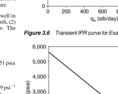
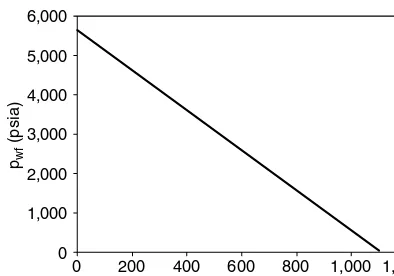
Figure 3.5: A typical IPR curve for an oil well. Figure 3.6: Transient IPR curve for Example Problem

3.1.

Figure 3.7: Steady-state IPR curve for Example Problem 3.1.

Figure 3.8: Pseudo–steady-state IPR curve for Example Problem 3.1.

Figure 3.9: IPR curve for Example Problem 3.2. Figure 3.10: Generalized Vogel IPR model for partial

two-phase reservoirs.

Figure 3.11: IPR curve for Example Problem 3.3. Figure 3.12: IPR curves for Example Problem 3.4,

Well A.

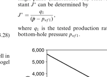
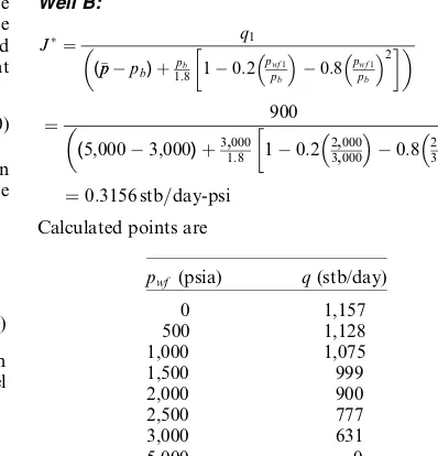
Figure 3.13: IPR curves for Example Problem 3.4, Well B

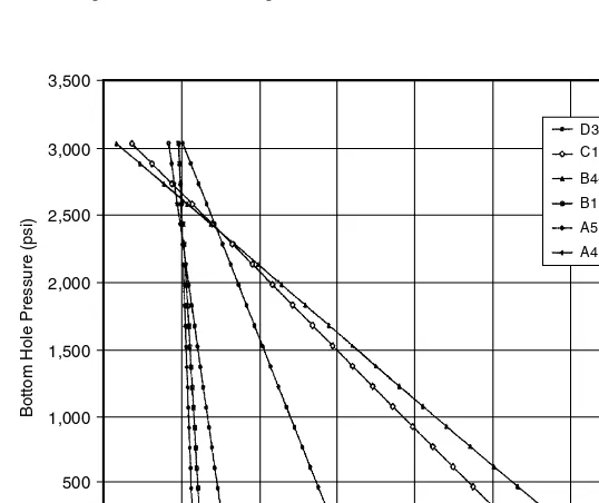
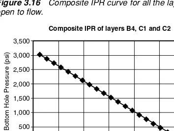
Figure 3.14: IPR curves for Example Problem 3.5. Figure 3.15: IPR curves of individual layers. Figure 3.16: Composite IPR curve for all the layers

open to flow.

Figure 3.17: Composite IPR curve for Group 2 (Layers B4, C1, and C2).

Figure 3.18: Composite IPR curve for Group 3 (Layers B1, A4, and A5).

Figure 3.19: IPR curves for Example Problem 3.6. Figure 3.20: IPR curves for Example Problem 3.7.

Figure 4.1: Flow along a tubing string.

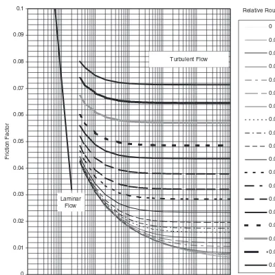
Figure 4.2: Darcy–Wiesbach friction factor diagram. Figure 4.3: Flow regimes in gas-liquid flow.

Figure 4.4: Pressure traverse given byHagedorn BrownCorreltion.xlsfor Example. Figure 4.5: Calculated tubing pressure profile for

Example Problem 4.5.

Figure 5.1: A typical choke performance curve. Figure 5.2: Choke flow coefficient for nozzle-type

chokes.

Figure 5.3: Choke flow coefficient for orifice-type chokes.

Figure 6.1: Nodal analysis for Example Problem 6.1. Figure 6.2: Nodal analysis for Example Problem 6.4. Figure 6.3: Nodal analysis for Example Problem 6.5. Figure 6.4: Nodal analysis for Example Problem 6.6. Figure 6.5: Nodal analysis for Example Problem 6.8. Figure 6.6: Schematic of a multilateral well trajectory. Figure 6.7: Nomenclature of a multilateral well. Figure 7.1: Nodal analysis plot for Example Problem

7.1.

Figure 7.2: Production forecast for Example Problem 7.2.

Figure 7.3: Nodal analysis plot for Example Problem 7.2.

Figure 7.4: Production forecast for Example Problem 7.2

Figure 7.3: Production forecast for Example Problem 7.3.

Figure 7.4: Result of production forecast for Example Problem 7.4.

Figure 8.1: A semilog plot ofqversustindicating an exponential decline.

Figure 8.2: A plot ofNpversusqindicating an exponential decline.

Figure 8.3: A plot of log(q) versus log(t) indicating a harmonic decline.

Figure 8.4: A plot ofNpversus log(q) indicating a harmonic decline.

Figure 8.5: A plot of relative decline rate versus production rate.

Figure 8.6: Procedure for determininga- andb-values. Figure 8.7: A plot of log(q) versustshowing an

exponential decline.

Figure 8.8: Relative decline rate plot showing exponential decline.

Figure 8.9: Projected production rate by an exponential decline model. Figure 8.10: Relative decline rate plot showing

harmonic decline.

Figure 8.11: Projected production rate by a harmonic decline model.

Figure 8.12: Relative decline rate plot showing hyperbolic decline.

Figure 8.13: Relative decline rate plot showing hyperbolic decline.

Figure 8.14: Projected production rate by a hyperbolic decline model.

Figure 9.1: A simple uniaxial test of a metal specimen. Figure 9.2: Effect of tension stress on tangential stress. Figure 9.3: Tubing–packer relation.

Figure 9.4: Ballooning and buckling effects. Figure 10.1: A typical vertical separator. Figure 10.2: A typical horizontal separator. Figure 10.3: A typical horizontal double-tube

separator.

Figure 10.5: A typical spherical low-pressure separator.

Figure 10.6: Water content of natural gases. Figure 10.7: Flow diagram of a typical solid desiccant

dehydration plant.

Figure 10.8: Flow diagram of a typical glycol dehydrator.

Figure 10.9: Gas capacity of vertical inlet scrubbers based on 0.7-specific gravity at 1008F. Figure 10.10: Gas capacity for trayed glycol contactors

based on 0.7-specific gravity at 1008F. Figure 10.11: Gas capacity for packed glycol

contactors based on 0.7-specific gravity at 1008F.

Figure 10.12: The required minimum height of packing of a packed contactor, or the minimum number of trays of a trayed contactor. Figure 11.1: Double-action stroke in a duplex pump. Figure 11.2: Single-action stroke in a triplex pump. Figure 11.3: Elements of a typical reciprocating

compressor.

Figure 11.4: Cross-section of a centrifugal compressor.

Figure 11.5: Basic pressure–volume diagram. Figure 11.6: Flow diagram of a two-stage

compression unit.

Figure 11.7: Fuel consumption of prime movers using three types of fuel.

Figure 11.8: Fuel consumption of prime movers using natural gas as fuel.

Figure 11.9: Effect of elevation on prime mover power.

Figure 11.10: Darcy–Wiesbach friction factor chart. Figure 11.11: Stresses generated by internal pressurep

in a thin-wall pipe,D=t>20.

Figure 11.12: Stresses generated by internal pressurep in a thick-wall pipe,D=t<20.

Figure 11.13: Calculated temperature profiles with a polyethylene layer of 0.0254 M (1 in.). Figure 11.14: Calculated steady-flow temperature

profiles with polyethylene layers of various thicknesses.

Figure 11.15: Calculated temperature profiles with a polypropylene layer of 0.0254 M (1 in.). Figure 11.16: Calculated steady-flow temperature

profiles with polypropylene layers of various thicknesses.

Figure 11.17: Calculated temperature profiles with a polyurethane layer of 0.0254 M (1 in.). Figure 11.18: Calculated steady-flow temperature

profiles with polyurethane layers of four thicknesses.

Figure 12.1: A diagrammatic drawing of a sucker rod pumping system.

Figure 12.2: Sketch of three types of pumping units: (a) conventional unit; (b) Lufkin Mark II unit; (c) air-balanced unit.

Figure 12.3: The pumping cycle: (a) plunger moving down, near the bottom of the stroke; (b) plunger moving up, near the bottom of the stroke; (c) plunger moving up, near the top of the stroke; (d) plunger moving down, near the top of the stroke. Figure 12.4: Two types of plunger pumps.

Figure 12.5: Polished rod motion for (a) conventional pumping unit and (b) air-balanced unit. Figure 12.6: Definitions of conventional pumping

unit API geometry dimensions. Figure 12.7: Approximate motion of connection point

between pitman arm and walking beam. Figure 12.8: Sucker rod pumping unit selection chart. Figure 12.9: A sketch of pump dynagraph.

Figure 12.10: Pump dynagraph cards: (a) ideal card, (b) gas compression on down-stroke, (c) gas expansion on upstroke, (d) fluid pound, (e) vibration due to fluid pound, (f) gas lock.

Figure 12.11: Surface Dynamometer Card: (a) ideal card (stretch and contraction), (b) ideal card (acceleration), (c) three typical cards.

Figure 12.12: Strain-gage–type dynamometer chart. Figure 12.13: Surface to down hole cards derived from

surface dynamometer card.

Figure 13.1: Configuration of a typical gas lift well. Figure 13.2: A simplified flow diagram of a closed

rotary gas lift system for single intermittent well.

Figure 13.3: A sketch of continuous gas lift. Figure 13.4: Pressure relationship in a continuous gas

lift.

Figure 13.5: System analysis plot given byGasLift Potential.xlsfor the unlimited gas injection case.

Figure 13.6: System analysis plot given byGasLift Potential.xlsfor the limited gas injection case.

Figure 13.7: Well unloading sequence. Figure 13.8: Flow characteristics of orifice-type

valves.

Figure 13.9: Unbalanced bellow valve at its closed condition.

Figure 13.10: Unbalanced bellow valve at its open condition.

Figure 13.11: Flow characteristics of unbalanced valves. Figure 13.12: A sketch of a balanced pressure valve. Figure 13.13: A sketch of a pilot valve.

Figure 13.14: A sketch of a throttling pressure valve. Figure 13.15: A sketch of a fluid-operated valve. Figure 13.16: A sketch of a differential valve. Figure 13.17: A sketch of combination valve. Figure 13.18: A flow diagram to illustrate procedure of

valve spacing.

Figure 13.19: Illustrative plot of BHP of an intermittent flow.

Figure 13.20: Intermittent flow gradient at mid-point of tubing.

Figure 13.21: Example Problem 13.8 schematic and BHP build.up for slug flow. Figure 13.22: Three types of gas lift installations. Figure 13.23: Sketch of a standard two-packer

chamber.

Figure 13.24: A sketch of an insert chamber. Figure 13.25: A sketch of a reserve flow chamber.

Figure 14.1: A sketch of an ESP installation. Figure 14.2: An internal schematic of centrifugal

pump.

Figure 14.3: A sketch of a multistage centrifugal pump.

Figure 14.4: A typical ESP characteristic chart. Figure 14.5: A sketch of a hydraulic piston pump. Figure 14.6: Sketch of a PCP system.

Figure 14.7: Rotor and stator geometry of PCP. Figure 14.8: Four flow regimes commonly

encountered in gas wells. Figure 14.9: A sketch of a plunger lift system. Figure 14.10: Sketch of a hydraulic jet pump

installation.

Figure 14.11: Working principle of a hydraulic jet pump.

Figure 14.12: Example jet pump performance chart. Figure 15.1: Temperature and spinner

Figure 15.3: Measured bottom-hole pressures and oil production rates during a pressure drawdown test.

Figure 15.4: Log-log diagnostic plot of test data. Figure 15.5: Semi-log plot for vertical radial flow

analysis.

Figure 15.6: Square-root time plot for pseudo-linear flow analysis.

Figure 15.7: Semi-log plot for horizontal pseudo-radial flow analysis.

Figure 15.8: Match between measured and model calculated pressure data.

Figure 15.9: Gas production due to channeling behind the casing.

Figure 15.10: Gas production due to preferential flow through high-permeability zones. Figure 15.11: Gas production due to gas coning. Figure 15.12: Temperature and noise logs identifying

gas channeling behind casing. Figure 15.13: Temperature and fluid density logs

identifying a gas entry zone. Figure 15.14: Water production due to channeling

behind the casing.

Figure 15.15: Preferential water flow through high-permeability zones.

Figure 15.16: Water production due to water coning. Figure 15.17: Prefracture and postfracture temperature

logs identifying fracture height. Figure 15.18: Spinner flowmeter log identifying a

watered zone at bottom.

Figure 15.19: Calculated minimum flow rates with Turner et al.’s model and test flow rates. Figure 15.20: The minimum flow rates given by Guo

et al.’s model and the test flow rates. Figure 16.1: Typical acid response curves.

Figure 16.2: Wormholes created by acid dissolution of limestone.

Figure 17.1: Schematic to show the equipment layout in hydraulic fracturing treatments of oil and gas wells.

Figure 17.2: A schematic to show the procedure of hydraulic fracturing treatments of oil and gas wells.

Figure 17.3: Overburden formation of a hydrocarbon reservoir.

Figure 17.4: Concept of effective stress between grains.

Figure 17.5: The KGD fracture geometry. Figure 17.6: The PKN fracture geometry. Figure 17.7: Relationship between fracture

conductivity and equivalent skin factor. Figure 17.8: Relationship between fracture

conductivity and equivalent skin factor. Figure 17.9: Effect of fracture closure stress on

proppant pack permeability. Figure 17.10: Iteration procedure for injection time

calculation.

Figure 17.11: Calculated slurry concentration. Figure 17.12: Bottom-hole pressure match with

three-dimensional fracturing model PropFRAC.

Figure 17.13: Four flow regimes that can occur in hydraulically fractured reservoirs. Figure 18.1: Comparison of oil well inflow

performance relationship (IPR) curves before and after stimulation. Figure 18.2: A typical tubing performance curve. Figure 18.3: A typical gas lift performance curve of a

low-productivity well.

Figure 18.4: Theoretical load cycle for elastic sucker rods.

Figure 18.5: Actual load cycle of a normal sucker rod. Figure 18.6: Dimensional parameters of a

dynamometer card.

Figure 18.7: A dynamometer card indicating synchronous pumping speeds.

Figure 18.8: A dynamometer card indicating gas lock. Figure 18.9: Sketch of (a) series pipeline and

(b) parallel pipeline. Figure 18.10: Sketch of a looped pipeline.

Figure 18.11: Effects of looped line and pipe diameter ratio on the increase of gas flow rate. Figure 18.12: A typical gas lift performance curve of

a high-productivity well.

Figure 18.13: Schematics of two hierarchical networks. Figure 18.14: An example of a nonhierarchical

Table of Contents

Preface

List of Symbols

List of Tables

List of Figures

Part I: Petroleum Production Engineering Fundamentals:

Chapter 1: Petroleum Production System

Chapter 2: Properties of Oil and Natural Gas

Chapter 3: Reservoir Deliverability

Chapter 4: Wellbore Performance

Chapter 5: Choke Performance

Chapter 6: Well Deliverability

Chapter 7: Forecast of Well Production

Chapter 8: Production Decline Analysis

Part II: Equipment Design and Selection

Chapter 9: Well Tubing

Chapter 10: Separation Systems

Chapter 12: Sucker Rod Pumping

Chapter 13: Gas Lift

Chapter 14: Other Artificial Lift Methods

Part IV: Production Enhancement

Chapter 15: Well Problem Identification

Chapter 16: Matrix Acidizing

Chapter 17: Hydraulic Fracturing

Chapter 18: Production Optimization

Appendix A: Unit Conversion Factors

Part I

Petroleum

Production

Engineering

Fundamentals

The upstream of the petroleum industry involves itself in the business of oil and gas exploration and production (E & P) activities. While the exploration activities find oil and gas reserves, the production activities deliver oil and gas to the downstream of the industry (i.e., processing plants). The petroleum production is definitely the heart of the petroleum industry.

Petroleum production engineering is that part of petroleum engineering that attempts to maxi-mize oil and gas production in a cost-effective manner. To achieve this objective, production engineers need to have a thorough understanding of the petroleum production systems with which they work. To perform their job correctly, production engineers should have solid back-ground and sound knowledge about the properties of fluids they produce and working principles of all the major components of producing wells and surface facilities. This part of the book provides graduating production engineers with fundamentals of petroleum production engineering. Materials are presented in the following eight chapters:

Chapter 1 Petroleum Production System 1/3 Chapter 2 Properties of Oil and Natural Gas 2/19 Chapter 3 Reservoir Deliverability 3/29

1

Petroleum

Production

System

Contents

1.1 Introduction 1/4 1.2 Reservoir 1/4 1.3 Well 1/5 1.4 Separator 1/8 1.5 Pump 1/9

1.6 Gas Compressor 1/10 1.7 Pipelines 1/11

1.8 Safety Control System 1/11 1.9 Unit Systems 1/17 Summary 1/17

1.1 Introduction

The role of a production engineer is to maximize oil and gas production in a cost-effective manner. Familiarization and understanding of oil and gas production systems are essential to the engineers. This chapter provides graduat-ing production engineers with some basic knowledge about production systems. More engineering principles are discussed in the later chapters.

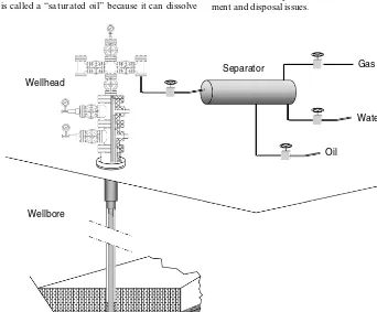
As shown in Fig. 1.1, a complete oil or gas production system consists of a reservoir, well, flowline, separators, pumps, and transportation pipelines. The reservoir sup-plies wellbore with crude oil or gas. The well provides a path for the production fluid to flow from bottom hole to surface and offers a means to control the fluid production rate. The flowline leads the produced fluid to separators. The separators remove gas and water from the crude oil. Pumps and compressors are used to transport oil and gas through pipelines to sales points.

1.2 Reservoir

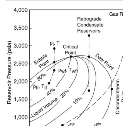
Hydrocarbon accumulations in geological traps can be clas-sified as reservoir, field, and pool. A ‘‘reservoir’’ is a porous and permeable underground formation containing an indi-vidual bank of hydrocarbons confined by impermeable rock or water barriers and is characterized by a single natural pressure system. A ‘‘field’’ is an area that consists of one or more reservoirs all related to the same structural feature. A ‘‘pool’’ contains one or more reservoirs in isolated structures. Depending on the initial reservoir condition in the phase diagram (Fig. 1.2), hydrocarbon accumulations are classi-fied as oil, gas condensate, and gas reservoirs. An oil that is at a pressure above its bubble-point pressure is called an ‘‘undersaturated oil’’ because it can dissolve more gas at the given temperature. An oil that is at its bubble-point pressure is called a ‘‘saturated oil’’ because it can dissolve

no more gas at the given temperature. Single (liquid)-phase flow prevails in an undersaturated oil reservoir, whereas two-phase (liquid oil and free gas) flow exists in a sat-urated oil reservoir.

Wells in the same reservoir can fall into categories of oil, condensate, and gas wells depending on the producing gas–oil ratio (GOR). Gas wells are wells with producing GOR being greater than 100,000 scf/stb; condensate wells are those with producing GOR being less than 100,000 scf/stb but greater than 5,000 scf/stb; and wells with producing GOR being less than 5,000 scf/stb are classified as oil wells.

Oil reservoirs can be classified on the basis of boundary type, which determines driving mechanism, and which are as follows:

. Water-drive reservoir . Gas-cap drive reservoir . Dissolved-gas drive reservoir

In water-drive reservoirs, the oil zone is connected by a continuous path to the surface groundwater system (aqui-fer). The pressure caused by the ‘‘column’’ of water to the surface forces the oil (and gas) to the top of the reservoir against the impermeable barrier that restricts the oil and gas (the trap boundary). This pressure will force the oil and gas toward the wellbore. With the same oil production, reservoir pressure will be maintained longer (relative to other mech-anisms of drive) when there is an active water drive. Edge-water drive reservoir is the most preferable type of reservoir compared to bottom-water drive. The reservoir pressure can remain at its initial value above bubble-point pressure so that single-phase liquid flow exists in the reservoir for maximum well productivity. A steady-state flow condition can prevail in a edge-water drive reservoir for a long time before water breakthrough into the well. Bottom-water drive reservoir (Fig. 1.3) is less preferable because of water-coning problems that can affect oil production economics due to water treat-ment and disposal issues.

Wellbore

Reservoir Separator Wellhead

P_wf P P_e

Gas

Oil

Water

In a gas-cap drive reservoir, gas-cap drive is the drive mechanism where the gas in the reservoir has come out of solution and rises to the top of the reservoir to form a gas cap (Fig. 1.4). Thus, the oil below the gas cap can be produced. If the gas in the gas cap is taken out of the reservoir early in the production process, the reservoir pressure will decrease rapidly. Sometimes an oil reservoir is subjected to both water and gas-cap drive.

A dissolved-gas drive reservoir (Fig. 1.5) is also called a ‘‘solution-gas drive reservoir’’ and ‘‘volumetric reservoir.’’ The oil reservoir has a fixed oil volume surrounded by no-flow boundaries (faults or pinch-outs). Dissolved-gas drive is the drive mechanism where the reservoir gas is held in

solution in the oil (and water). The reservoir gas is actually in a liquid form in a dissolved solution with the liquids (at atmospheric conditions) from the reservoir. Compared to the water- and gas-drive reservoirs, expansion of solution (dissolved) gas in the oil provides a weak driving mech-anism in a volumetric reservoir. In the regions where the oil pressure drops to below the bubble-point pressure, gas escapes from the oil and oil–gas two-phase flow exists. To improve oil recovery in the solution-gas reservoir, early pressure maintenance is usually preferred.

1.3 Well

Oil and gas wells are drilled like an upside-down telescope. The large-diameter borehole section is at the top of the well. Each section is cased to the surface, or a liner is placed in the well that laps over the last casing in the well. Each casing or liner is cemented into the well (usually up to at least where the cement overlaps the previous cement job).

The last casing in the well is the production casing (or production liner). Once the production casing has been cemented into the well, the production tubing is run into the well. Usually a packer is used near the bottom of the tubing to isolate the annulus between the outside of the tubing and the inside of the casing. Thus, the produced fluids are forced to move out of the perforation into the bottom of the well and then into the inside of the tubing. Packers can be actuated by either mechanical or hydraulic mechanisms. The production tubing is often (particularly during initial well flow) provided with a bottom-hole choke to control the initial well flow (i.e., to restrict over-production and loss of reservoir pressure).

Figure 1.6 shows a typical flowing oil well, defined as a well producing solely because of the natural pressure of the reservoir. It is composed of casings, tubing, packers, down-hole chokes (optional), wellhead, Christmas tree, and surface chokes.

0 50 100 150 200 250 300 350

1,000

500 1,500 2,000 2,500 3,000 3,500 4,000

Reservoir Temperature (⬚F)

Reservoir Pressure (psia)

Liquid Volume 40% _20%

10% 80%

5% 0%

Bubble Point

Gas Reservoirs Retrograde

Condensate Reservoirs

Critical Point pi, T

ptf, Ttf

pwf, Twf

Dew Point

Cricondentherm

Point

Figure 1.2 A typical hydrocarbon phase diagram.

Water WOC

Oil

Most wells produce oil through tubing strings, mainly because a tubing string provides good sealing performance and allows the use of gas expansion to lift oil. The Ameri-can Petroleum Institute (API) defines tubing size using nominal diameter and weight (per foot). The nominal diameter is based on the internal diameter of the tubing body. The weight of tubing determines the tubing outer diameter. Steel grades of tubing are designated H-40, J-55, C-75, L-80, N-80, C-90, and P-105, where the digits repre-sent the minimum yield strength in 1,000 psi. The min-imum performance properties of tubing are given in Chapter 9 and Appendix B.

The ‘‘wellhead’’ is defined as the surface equipment set below the master valve. As we can see in Fig. 1.7, it includes casing heads and a tubing head. The casing head (lowermost) is threaded onto the surface casing. This can also be a flanged or studded connection. A ‘‘casing head’’ is a mechanical assembly used for hanging a casing string (Fig. 1.8). Depending on casing programs in well drilling, several casing heads can be installed during well construc-tion. The casing head has a bowl that supports the casing hanger. This casing hanger is threaded onto the top of the production casing (or uses friction grips to hold the cas-ing). As in the case of the production tubing, the produc-tion casing is landed in tension so that the casing hanger actually supports the production casing (down to the freeze point). In a similar manner, the intermediate cas-ing(s) are supported by their respective casing hangers (and bowls). All of these casing head arrangements are supported by the surface casing, which is in compression and cemented to the surface. A well completed with three casing strings has two casing heads. The uppermost casing head supports the production casing. The lowermost cas-ing head sits on the surface cascas-ing (threaded to the top of the surface casing).

Most flowing wells are produced through a string of tubing run inside the production casing string. At the surface, the tubing is supported by the tubing head (i.e., the tubing head is used for hanging tubing string on the production casing head [Fig. 1.9]). The tubing head sup-ports the tubing string at the surface (this tubing is landed on the tubing head so that it is in tension all the way down to the packer).

The equipment at the top of the producing wellhead is called a ‘‘Christmas tree’’ (Fig. 1.10) and it is used to control flow. The ‘‘Christmas tree’’ is installed above the tubing head. An ‘‘adaptor’’ is a piece of equipment used to join the two. The ‘‘Christmas tree’’ may have one flow outlet (a tee) or two flow outlets (a cross). The master valve is installed below the tee or cross. To replace a master valve, the tubing must be plugged. A Christmas tree consists of a main valve, wing valves, and a needle valve. These valves are used for closing the well when needed. At the top of the tee structure (on the top of the ‘‘Christmas tree’’), there is a pressure gauge that indicates the pressure in the tubing.

Gas Cap

Oil

Figure 1.4 A sketch of a gas-cap drive reservoir.

Oil and Gas

Reservoir

The wing valves and their gauges allow access (for pressure measurements and gas or liquid flow) to the annulus spaces (Fig. 1.11).

‘‘Surface choke’’ (i.e., a restriction in the flowline) is a piece of equipment used to control the flow rate (Fig. 1.12). In most flowing wells, the oil production rate is altered by adjusting the choke size. The choke causes back-pressure

in the line. The back-pressure (caused by the chokes or other restrictions in the flowline) increases the bottom-hole flowing pressure. Increasing the bottom-bottom-hole flowing pressure decreases the pressure drop from the reservoir to the wellbore (pressure drawdown). Thus, increasing the back-pressure in the wellbore decreases the flow rate from the reservoir.

In some wells, chokes are installed in the lower section of tubing strings. This choke arrangement reduces well-head pressure and enhances oil production rate as a result of gas expansion in the tubing string. For gas wells, use of down-hole chokes minimizes the gas hydrate problem in the well stream. A major disadvantage of using down-hole chokes is that replacing a choke is costly.

Certain procedures must be followed to open or close a well. Before opening, check all the surface equipment such as safety valves, fittings, and so on. The burner of a line heater must be lit before the well is opened. This is neces-sary because the pressure drop across a choke cools the fluid and may cause gas hydrates or paraffin to deposit out. A gas burner keeps the involved fluid (usually water) hot. Fluid from the well is carried through a coil of piping. The choke is installed in the heater. Well fluid is heated both before and after it flows through the choke. The upstream heating helps melt any solids that may be present in the producing fluid. The downstream heating prevents hydrates and paraffins from forming at the choke.

Surface vessels should be open and clear before the well is allowed to flow. All valves that are in the master valve and other downstream valves are closed. Then follow the following procedure to open a well:

1. The operator barely opens the master valve (just a crack), and escaping fluid makes a hissing sound. When the fluid no longer hisses through the valve, the pressure has been equalized, and then the master valve is opened wide.

2. If there are no oil leaks, the operator cracks the next downstream valve that is closed. Usually, this will be Casing Perforation

Wellhead

Oil Reservoir Packer

Bottom-hole Choke Tubing

Annulus

Production Casing Intermediate Casing Surface Casing

Cement

Wellbore

Reservoir

Figure 1.6 A sketch of a typical flowing oil well.

Choke

Wing Valve

Master Valve Tubing Pressure Gauge

Flow Fitting

Tubing

Intermediate Casing

Surface Casing Lowermost Casing Head

Uppermost Casing Head Casing Valve

Casing Pressure Gauge

Production Casing Tubing Head

either the second (backup) master valve or a wing valve. Again, when the hissing sound stops, the valve is opened wide.

3. The operator opens the other downstream valves the same way.

4. To read the tubing pressure gauge, the operator must open the needle valve at the top of the Christmas tree. After reading and recording the pressure, the operator may close the valve again to protect the gauge.

The procedure for ‘‘shutting-in’’ a well is the opposite of the procedure for opening a well. In shutting-in the well, the master valve is closed last. Valves are closed rather rapidly to avoid wearing of the valve (to prevent erosion). At least two valves must be closed.

1.4 Separator

The fluids produced from oil wells are normally complex mixtures of hundreds of different compounds. A typical oil well stream is a high-velocity, turbulent, constantly expanding mixture of gases and hydrocarbon liquids, in-timately mixed with water vapor, free water, and some-times solids. The well stream should be processed as soon as possible after bringing them to the surface. Separators are used for the purpose.

Three types of separators are generally available from manufacturers: horizontal, vertical, and spherical sep-arators. Horizontal separators are further classified into

Bowl

Production Casing

Casing Head

Surface Casing Casing Hanger

Figure 1.8 A sketch of a casing head.

Bowl

Seal

Tubing Hanger

Tubing Head

Figure 1.9 A sketch of a tubing head.

Choke Wing Valve

Wing Valve Choke

Master Valve

Tubing Head Adaptor Swabbing Valve Top Connection Gauge Valve

Flow Fitting

two categories: single tube and double tube. Each type of separator has specific advantages and limitations. Selec-tion of separator type is based on several factors including characteristics of production steam to be treated, floor space availability at the facility site, transportation, and cost.

Horizontal separators (Fig. 1.13) are usually the first choice because of their low costs. Horizontal separators are almost widely used for high-GOR well streams, foam-ing well streams, or liquid-from-liquid separation. They have much greater gas–liquid interface because of a large, long, baffled gas-separation section. Horizontal sep-arators are easier to skid-mount and service and require less piping for field connections. Individual separators can be stacked easily into stage-separation assemblies to min-imize space requirements. In horizontal separators, gas flows horizontally while liquid droplets fall toward the liquid surface. The moisture gas flows in the baffle surface and forms a liquid film that is drained away to the liquid section of the separator. The baffles need to be longer than the distance of liquid trajectory travel. The liquid-level control placement is more critical in a horizontal separator than in a vertical separator because of limited surge space. Vertical separators are often used to treat low to inter-mediate GOR well streams and streams with relatively large slugs of liquid. They handle greater slugs of liquid without carryover to the gas outlet, and the action of the liquid-level control is not as critical. Vertical separators occupy less floor space, which is important for facility sites

such as those on offshore platforms where space is limited. Because of the large vertical distance between the liquid level and the gas outlet, the chance for liquid to re-vapor-ize into the gas phase is limited. However, because of the natural upward flow of gas in a vertical separator against the falling droplets of liquid, adequate separator diameter is required. Vertical separators are more costly to fabricate and ship in skid-mounted assemblies.

Spherical separators offer an inexpensive and compact means of separation arrangement. Because of their com-pact configurations, these types of separators have a very limited surge space and liquid-settling section. Also, the placement and action of the liquid-level control in this type of separator is more critical.

Chapter 10 provides more details on separators and dehydrators.

1.5 Pump

After separation, oil is transported through pipelines to the sales points. Reciprocating piston pumps are used to provide mechanical energy required for the transportation. There are two types of piston strokes, the single-action

Handwheel

Packing

Gate

Port

Figure 1.11 A sketch of a surface valve.

Wellhead Choke

Figure 1.12 A sketch of a wellhead choke.

piston stroke and the double-action piston stroke. The double-action stroke is used for duplex (two pistons) pumps. The single-action stroke is used for pumps with three pistons or greater (e.g., triplex pump). Figure 1.14 shows how a duplex pump works. More information about pumps is presented in Chapter 11.

1.6 Gas Compressor

Compressors are used for providing gas pressure required to transport gas with pipelines and to lift oil in gas-lift operations. The compressors used in today’s natural gas production industry fall into two distinct types: reciprocat-ing and rotary compressors. Reciprocatreciprocat-ing compressors are most commonly used in the natural gas industry. They are built for practically all pressures and volumetric capacities.

As shown in Fig. 1.15, reciprocating compressors have more moving parts and, therefore, lower mechanical efficiencies than rotary compressors. Each cylinder assembly of a recip-rocating compressor consists of a piston, cylinder, cylinder heads, suction and discharge valves, and other parts neces-sary to convert rotary motion to reciprocation motion. A reciprocating compressor is designed for a certain range of compression ratios through the selection of proper piston displacement and clearance volume within the cylinder. This clearance volume can be either fixed or variable, depending on the extent of the operation range and the percent of load variation desired. A typical reciprocating compressor can deliver a volumetric gas flow rate up to 30,000 cubic feet per minute (cfm) at a discharge pressure up to 10,000 psig.

Rotary compressors are divided into two classes: the centrifugal compressor and the rotary blower. A

centrifu-Discharge centrifu-Discharge

P₂

P₁ P₁

P₂

Piston Rod

Suction Suction

d_L

d_r

L_s

Piston

Figure 1.14 Double-action piston pump.

Piston Rod

Wrist Pin

Suction Valve

Discharge Valve

Cylinder Head

Cylinder Crosshead

Connecting Rod

Crankshaft

Piston

gal compressor consists of a housing with flow passages, a rotating shaft on which the impeller is mounted, bearings, and seals to prevent gas from escaping along the shaft. Centrifugal compressors have few moving parts because only the impeller and shaft rotate. Thus, its efficiency is high and lubrication oil consumption and maintenance costs are low. Cooling water is normally unnecessary be-cause of lower compression ratio and less friction loss. Compression rates of centrifugal compressors are lower because of the absence of positive displacement. Centrifu-gal compressors compress gas using centrifuCentrifu-gal force. In this type of compressor, work is done on the gas by an impeller. Gas is then discharged at a high velocity into a diffuser where the velocity is reduced and its kinetic energy is converted to static pressure. Unlike reciprocating com-pressors, all this is done without confinement and physical squeezing. Centrifugal compressors with relatively unre-stricted passages and continuous flow are inherently high-capacity, low-pressure ratio machines that adapt easily to series arrangements within a station. In this way, each compressor is required to develop only part of the station compression ratio. Typically, the volume is more than 100,000 cfm and discharge pressure is up to 100 psig. More information about different types of compressors is provided in Chapter 11.

1.7 Pipelines

The first pipeline was built in the United States in 1859 to transport crude oil (Wolbert, 1952). Through the one and half century of pipeline operating practice, the petro-leum industry has proven that pipelines are by far the

most economical means of large-scale overland transpor-tation for crude oil, natural gas, and their products, clearly superior to rail and truck transportation over competing routes, given large quantities to be moved on a regular basis. Transporting petroleum fluids with pipelines is a continuous and reliable operation. Pipelines have demonstrated an ability to adapt to a wide variety of environments including remote areas and hostile environ-ments. With very minor exceptions, largely due to local peculiarities, most refineries are served by one or more pipelines, because of their superior flexibility to the alternatives.

Figure 1.16 shows applications of pipelines in offshore operations. It indicates flowlines transporting oil and/or gas from satellite subsea wells to subsea manifolds, flow-lines transporting oil and/or gas from subsea manifolds to production facility platforms, infield flowlines transport-ing oil and/or gas from between production facility plat-forms, and export pipelines transporting oil and/or gas from production facility platforms to shore.

The pipelines are sized to handle the expected pressure and fluid flow. To ensure desired flow rate of product, pipeline size varies significantly from project to project. To contain the pressures, wall thicknesses of the pipelines range from3⁄8inch to 11⁄2inch. More information about pipelines is provided in Chapter 11.

1.8 Safety Control System

The purpose of safety systems is to protect personnel, the environment, and the facility. The major objective of the safety system is to prevent the release of hydrocarbons

Expansion Tie-in Spoolpiece

Infield Flowline

Riser

Tie-in

Subsea Manifold

Flowlines (several can be bundled) Satellite

Subsea Wells

Flowlines

Export Pipeline Existing Line

Pipeline Crossing

To Shore