Informasi Dokumen
- Penulis:
- M. Scutari
- J.-B. Denis
- Sekolah: UCL Genetics Institute
- Mata Pelajaran: Genetics
- Topik: Bayesian Networks: With Examples in R
- Tipe: book
- Tahun: 2015
- Kota: London
Ringkasan Dokumen
I. The Discrete Case: Multinomial Bayesian Networks
This chapter introduces the fundamental concepts of Bayesian Networks (BNs) using a hypothetical transport survey. The focus is on modeling discrete data, with continuous data and more complex data types addressed in subsequent chapters. The chapter systematically guides the reader through building and interpreting a BN, emphasizing the practical application of the theoretical principles.
1.1 Introductory Example: Train Use Survey
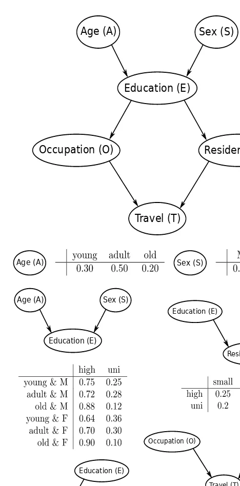
This section introduces a hypothetical survey investigating transport usage patterns, focusing on cars and trains. Six discrete variables are defined: Age, Sex, Education, Occupation, Residence, and Travel. These variables are categorized into demographic and socioeconomic indicators, with Travel as the target variable. The example's context is relevant for understanding the practical applications of BNs in analyzing survey data and drawing inferences about relationships between variables.
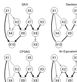
1.2 Graphical Representation
This section details the representation of variable relationships using a directed acyclic graph (DAG). Each node represents a variable, and arcs represent direct dependencies. The concepts of parents, children, paths, and cycles are explained. The use of the bnlearn R package is introduced for creating and manipulating DAGs, illustrating the practical steps involved in constructing the graphical representation of a BN. The example uses the empty.graph, set.arc, and modelstring functions within bnlearn to build the DAG step-by-step, demonstrating how direct dependencies are coded within the graph.
1.3 Probabilistic Representation
Here, the joint probability distribution over the variables is defined. The concept of the global distribution is introduced, followed by the factorization of this distribution into smaller, local distributions based on the DAG's conditional independence relationships. This factorization greatly reduces the number of parameters, a key advantage of BNs. The section demonstrates how to define local distributions using R's array and matrix functions, creating conditional probability tables (CPTs) for each variable. The code illustrates the creation of CPTs for variables with different numbers of parents, showing how to specify probabilities within the tables, thus defining the probabilistic component of the BN model.
1.4 Estimating the Parameters: Conditional Probability Tables
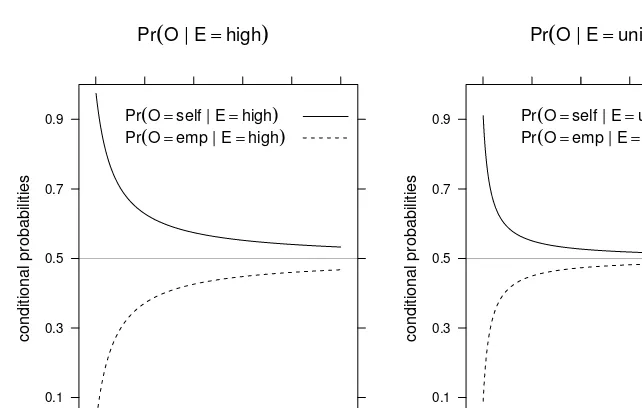
This section focuses on estimating the parameters (conditional probabilities) of the local distributions from observed data. Maximum likelihood estimation (MLE) using empirical frequencies is described, demonstrated with R code using the bn.fit function from the bnlearn package. Bayesian estimation, offering a more robust alternative to MLE, is introduced and illustrated, highlighting the role of the prior distribution and the imaginary sample size (iss) parameter in influencing posterior estimates. The concept of smoothing conditional probabilities to avoid sparse tables and improve prediction is discussed, showing the effect of varying the iss value on the resulting estimates.
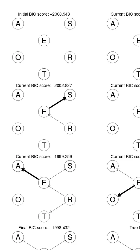
1.5 Learning the DAG Structure: Tests and Scores
This section addresses the scenario where the DAG structure is unknown and needs to be learned from data. This is a common task in fields like genetics and systems biology, where inferring network structures is crucial. The challenges of learning DAG structures are briefly introduced, setting the stage for a deeper discussion of structure learning algorithms in later chapters. The section touches on the use of conditional independence tests and network scores as methods for structure learning, creating a bridge to the more detailed theoretical exposition in Chapter 4.
1.6 Using Discrete BNs
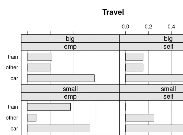
This section delves into the practical application of discrete BNs, focusing on how to use the DAG structure and the CPTs for inference. Exact and approximate inference methods are briefly introduced, providing a foundation for the more in-depth treatment of inference algorithms in Chapter 4. This section connects the theoretical aspects of BNs to their practical use in making predictions and drawing inferences from the model.
1.7 Plotting BNs
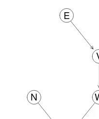
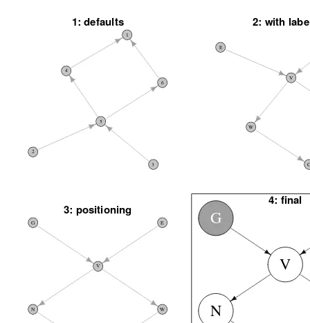
This section describes how to visually represent the learned BNs, focusing on plotting both the DAG structure and the CPTs. This visualization helps in understanding the network's relationships and the probability distributions associated with each node. While specific R code for plotting may not be explicitly detailed, the importance of visualization in understanding and communicating BN models is highlighted.
1.8 Further Reading
This section provides pointers to further reading on the topics covered in the chapter, directing readers to more advanced resources for a deeper understanding of discrete Bayesian Networks.
II. The Continuous Case: Gaussian Bayesian Networks
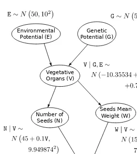
This chapter extends the concepts introduced in Chapter 1 to handle continuous data using Gaussian Bayesian Networks. Similar steps are followed, but the probabilistic representation is now based on Gaussian distributions and the focus shifts to correlation coefficients instead of conditional probability tables.
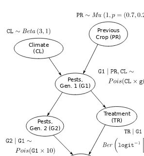
III. More Complex Cases: Hybrid Bayesian Networks
This chapter addresses the modeling of more complex scenarios involving hybrid Bayesian networks that contain a mixture of discrete and continuous variables. Strategies for handling such mixed data types are presented, including techniques for discretizing continuous variables and using different probability distributions.
IV. Theory and Algorithms for Bayesian Networks
This chapter delves into the theoretical foundations of Bayesian Networks, covering topics such as conditional independence, graphical separation, Markov blankets, moral graphs, and structure and parameter learning algorithms. Inference methods and causal Bayesian networks are also discussed, providing a more rigorous mathematical treatment of the subject matter.
V. Software for Bayesian Networks
This chapter provides an overview of available software packages for working with Bayesian Networks, focusing on R packages such as bnlearn, deal, catnet, and pcalg, as well as other software like BUGS, BayesiaLab, Hugin, and GeNIe.
VI. Real-World Applications of Bayesian Networks
This chapter presents real-world applications of Bayesian Networks in diverse fields. Two case studies are analyzed in detail to illustrate the practical use of BNs in solving real-world problems.
VII. Graph Theory
This appendix provides background information on graph theory, covering basic definitions and concepts relevant to understanding the graphical representation of Bayesian Networks.
VIII. Probability Distributions
This appendix reviews relevant probability distributions, including discrete and continuous distributions, and their properties. This section provides the necessary background in probability theory for understanding the probabilistic aspects of Bayesian Networks.
IX. A Note about Bayesian Networks
This appendix clarifies the relationship between Bayesian Networks and Bayesian statistics, addressing potential misconceptions.
Referensi Dokumen
- Categorical Data Analysis ( Agresti, A. )
- Local Causal and Markov Blanket Induction for Causal Discovery and Feature Selection for Classification Part I: Algorithms and Empirical Evaluation ( Aliferis, C. F., Statnikov, A., Tsamardinos, I., Mani, S., and Xenofon, X. D. )
- HUGIN – a Shell for Building Bayesian Belief Universes for Expert Systems ( Andersen, S., Olesen, K., Jensen, F., and Jensen, F. )
- An Introduction to Multivariate Statistical Analysis ( Anderson, T. W. )
- Probability and Measure Theory ( Ash, R. B. )