_________________________________________________________________________________________ Corresponding Author: F. Pasila, Electrical Engineering Department, Petra Christian University, Surabaya 60236, INDONESIA. Email:[email protected]
December 12 – 13, Ayodya Resort Bali, Indonesia
Multivariate Inputs on a MIMO Neuro-Fuzzy structure with LMA training. A study case: Indonesian Banking Stock Market
F. Pasila, R. Lim, M. Santoso
Electrical Engineering Department, Petra Christian University, Surabaya, 60236, INDONESIA
___________________________________________________________________________
Abstract: The paper describes the design and implementation of the multivariate inputs of multi-input-multi-output neuro-fuzzy with Levenberg-Marquardt algorithm training (MIMO neuro-fuzzy with accelerated LMA) to forecast stock market of Indonesian Banking. The accelerated LMA is efficient in the sense that it can bring the performance index of the network, such as the root mean squared error (RMSE), down to the desired error goal, more efficiently than the standard Levenberg-Marquardt algorithm. The MIMO neuro-fuzzy method is a hybrid intelligent system which combines the human-like reasoning style of fuzzy systems with the learning ability of neural nets. The main advantages of a MIMO neuro-fuzzy system are: it interprets IF-THEN rules from input-output relations and focuses on accuracy of the output network and offers efficient time consumption for on-line computation. The proposed architectures of this paper are a MIMO-neuro-fuzzy structure with multivariate input such as fundamental quantities as inputs network (High, Low, Open and Close) and a MIMO-neuro-fuzzy structure with other multivariate inputs, which is a combination inputs between two fundamental quantities (High and Low) and two inputs from technical indicator Exponential Moving Average (EMA High and EMA Low). Both proposed learning procedures, which are using accelerated LMA with optimal training parameters with at least one million iterations with different 16 membership functions, employ 12% of the input-output correspondences from the known input-output dataset. For experimental database, both structures are trained using the seven-year period (training data from 2 Oct 2006 to 28 Sept 2012) and tested using two-weeks period of the stock price index (prediction data from 1 Oct 2012 to 16 Oct 2012) and the proposed models are evaluated with a performance indicator, root mean squared error (RMSE) for mid-term forecasting application. The simulation results show that the MIMO-neuro-fuzzy structure with combination of fundamental quantities and technical indicators has better performance (RMSE) for two-weeks forecast.
Key words: MIMO neuro-fuzzy; accelerated Levenberg-Marquardt algorithm; multivariate inputs, fundamental quantities; technical indicator;
INTRODUCTION
As the arising of artificial intelligence algorithms in recent years, many researchers have applied soft computing algorithms in time-series model for financial forecasting. Some examples of the time-series forecasts can be seen below: Research of Kimoto, Asakawa, Yoda, and Takeoka (1990) developed a prediction system for stock market by using neural network; Nikolopoulos and Fellrath (1994) have combined genetic algorithms (GAs) and neural network (NN) to develop a hybrid expert system for investment decisions; Kim and Han (2000) proposed an approach based on genetic algorithms to feature discretization and the determination of connection weights for artificial neural networks (ANNs) to forecast the stock price index; Huarng and Yu (2006) applied a backpropagation neural network to establish fuzzy relationships in fuzzy time series for forecasting stock price; Moreover, Roh (2007) has combined neural network and time series model for forecasting the volatility of stock market index. In addition, another forecast strategy is done by Wei (2011), by proposing an adaptive-network-based fuzzy inference system model which uses multi-technical indicators and fundamental quantities, to predict stock price trends.
Even though most of the proposed solution schemes are formally very elegant and quite effective in forecasting the stock index, the problem of limited forecast (short-term forecasting) still remain.
A MIMO NEURO-FUZZY SYSTEM FOR MODELING AND FORECASTING
A neuro-fuzzy network with an improved training algorithm for MIMO case was developed by Palit and Popovic (2005) and used for forecasting of electrical load data.
/
Fig.1: The multivariate Architecture of the MIMO – feedforward Neuro-Fuzzy (NF) Network, type Takagi-Sugeno (TS)
The first proposed model of NF network as shown in Fig. 1 is based on Gaussian functions. It uses TS-fuzzy rule, product inference, and weighted average defuzzification. The nodes in the first layer compute the degree of membership of the fundamental input values (High, Low, Open and Close) in the antecedent fuzzy sets. The product nodes (x) denote the antecedent conjunction operator and the output of this node is the corresponding to degree of fulfillment or firing strength of the rule. The division (/), together with summation nodes (+), join to make the normalized degree of fulfillment (zl/b) of the corresponding rules, which after multiplication with the corresponding
TS rule consequent ( l j
y ), is used as input to the last summation part (+) at the defuzzyfied output value, which, being
crisp, is directly compatible with the next forecast data (High, Low, Open and Close).
The second model is also based on Fig. 1 but with combination between fundamental quantities and technical indicator in the input and output sides (multivariate inputs). The input XOPEN and XCLOSE will be replaced by input XEMA_HIGH
and
LOW EMA
X _ . The same changes also should be done in the output side.
1. NEURAL NETWORK REPRESENTATION OF FUZZY SYSTEM (FS)
Neuro-fuzzy representation of the FS is based on inference TS-type which has been explained clearly by Palit (p.153, p.233). There are two important steps in this representation: calculating of the degree of fulfillment and normalized degree of fulfillment. The FS considered here for constructing neuro-fuzzy structures is based on TS-type fuzzy model with Gaussian membership functions. It uses product inference rules and a weighted average defuzzifier defines as:
The corresponding lth rule from the above FS can be written as
m l mj l
j l oj j l
l m m l l
l
x W x W W y then
G is x and G is x and G is x If R
... ...
1 1
2 2 1 1
(1)
Where, xi withi1,2,...,m; and fj with j1,2,...,n; are the m system inputs and n system outputs, and ;
,..., 2 ,
1 m
i with Gl
i andl1,2,...,M;are the Gaussian membership functions of the form (1) with the corresponding
mean and variance parameters l i
c and
ilrespectively and with l jy as the output consequent of the lthrule.
network, where instead of the connection weights and the biases in training algorithm. We introduce the mean ciland the variance ilparameters of Gaussian functions, along with ijl
l ojW
W , parameters from the rules consequent, as the equivalent adjustable parameters of TS-type network. If all the parameters for NF network are properly selected, then the FS can correctly approximate any nonlinear system based on given related data between four inputs and four outputs.
M l
l l j
j y H
F
1
(2)
m l mj l
j l
j l
j l
j W W x W x W x
y 0 1 1 2 2... (3)
z bHl l/ , and
M l
l
Z b
1
(4)
m
i il
l i i
l x c
Z
1
2 exp
(5)
Prior to their use, NFTS and NFLUT models require the tuning of the parameters cnj,
nj, w0ni, wnji (for j = 1, 4; i = 1,4;). Here, the number of parameters for the considered MPRs is 252 parameters. The values of these parameters are found by an optimized learning procedure. The learning procedure employs 12% of the input-outputXIO correspondences from the known dataset.
2. ACCELERATED LEVENBERG-MARQUARDT ALGORITHM (LMA)
We introduce a function V
w is meant to minimize with respect to the parameter vector w using Newton’s method,the update of parameter vector w is defined as:
V w
V
ww
2 1
(6a)
k
wk ww 1 (6b)
From equation (6a), 2V
wis the Hessian matrix and V
w is the gradient of function
wV . If the V
w istaken to be SSE function as follows:
w e
w VN
r r
! 2
5 .
0 (7)
Then the gradient ofV
w and the hessian matrix of 2V
w are generally defined as:
w J
w e wV T r
(8a)
w J
w J w e
w e
wV r
N r
r
T 2
1
2
(8b) where J
w is the Jacobian matrix, written as follows
A A A
N N N
N
N N
w w e w
w e w
w e
w w e w
w e w
w e
w w e w
w e w
w e
w J
2 1
2
2 2
1 2
1
2 1
1 1
From (8c), it is seen that the dimension of the Jacobian matrix is (NNA), where N is the number of training models
and NA is the number of adjustable parameters in the network. For the Gauss-Newton method, the second term in (8b)
is assumed to be zero. Consequently, the update equations according to (6a) will be:
J w J w
J
w e ww r
T
T
1
(9a) Now let us see the LMA modifications of the Gauss-Newton method.
J w J w I
J
w e ww T T r
1 (9b)
where dimension of I is the (NANA) identity matrix, and the parameter is multiplied or divided by some factor
whenever the iteration steps increase or decrease the value of V w.
Here, the updated equation according to (6a)
k
wk
J
w J w I
J
w e ww r
T
T
1
1 (9c)
This is important to know that for large, the algorithm becomes the steepest descent algorithm with step size
/
1 , and for small, it becomes the Gauss-Newton method.
Now, comes to the computation of Jacobian Matrices. The gradient V
W0lj SSEcan be written as
j j
l l
j l
j S W Z b X d
W
V
0 / 0 / (10)
Where Xj and dj are the actual output of the Takagi-Sugeno type MIMO and the corresponding desired output
from matrix input-output training data. And then by comparing (8) to (9a), where the gradient V
w is expressed with the transpose of the Jacobian matrix multiplied with the network's error vector,
w J
w e wV T r
(11)
then the Jacobian matrix for the parameter W0lj, l ij
W , cil and l i
of the NF network can be written by
l
T l Tj T l
j J W Z b
W
J 0 0 / (12)
T i l T l ij T lij J W Z b x
W
J / (13)
l Ti l i i l eqv T
l i T l
i J c D Z x c
c J
2
/
2 (14)
l T i l i i l eqv Tl i T l
i J D Z x c
J 2 2/ 3 (15)
Where
12 2 2 1 1
p
eqv n n n
eqv f X f X e f X e e
D (16)
is a matrix form using pseudo inverse and
2 2 2
2 1
p n p p p
eqv e e e
e (17)
is sum square error with p = 1,2,3,...,N training samples that explained in Palit (2005) clearly. After finishing all computation in the (12-15), then back to the Eq. (6.b) for updating the four matrix parameters. The updating procedure will stop after achieving the maximum iteration or founding the minimum error function.
3. PROPOSED INPUT-OUTPUT RELATION FOR NF MODEL
The input data of the second model are HIGH, LOW, EMA HIGH and EMA LOW. The term EMA here is an Exponential Moving Average with ten times of period for each EMA HIGH and EMA LOW respectively. The related matrix between inputs and outputs of the MIMO Neuro-Fuzzy predictor of the first case should be arranged on XIO matrix, as shown below:
10 10 10 10 9 9 9 9 1 2 2 2 1 1 1 1 1 1 1 1 ... ... ... ... ... ... ... ... C O L H C O L H C O L H C O L H C O L H C O L H I Day Day Day Day Day Day Day Day Day Day Day Day Day Day Day Day Day Day Day Day Day Day Day Day XIO (18a) 10 10 10 10 9 9 9 9 2 2 2 2 1 1 1 1 1 1 1 1 ... ... ... ... ... ... ... ... L H L H L H L H L H L H L H L H L H L H L H L H II EMA EMA Day Day EMA EMA Day Day EMA EMA Day Day EMA EMA Day Day EMA EMA Day Day EMA EMA Day Day XIO (18b)
As shown in equation (18a), 4 input days (the last training data for inputs) are trained to produce 4 output days in NF network. Each input and output represents one daily set of data. Output from the first forecast
1 L1 O1 C1
H Day Day Day
Day will replace the 2nd row of XIOI as input for second prediction. After 10 loops of
forecasting, all ten outputs (in the right side) are output prediction of the next day until the next ten days of the related stock market. The same procedure above is done for the second case, with the matrix XIOIIshown in (18b). So far,
both matrix XIOare found optimal in the experimental procedures using optimal training parameters with at least one
million iterations with different 16 membership functions (from M = 5 until M = 15).
RESULT AND DISCUSSION
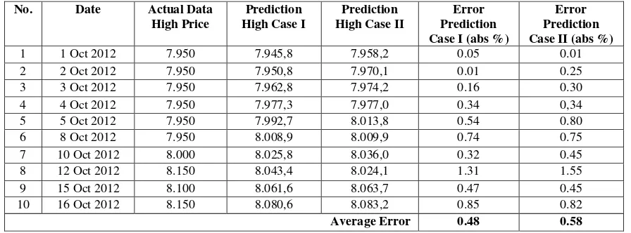
Tabel 1. Mid-Term Performance of NF Case I and II for BBCA (Data Training 2 Oct 2006 – 28 Sept 2012)
No. Date Actual Data
High Price
Prediction High Case I
Prediction High Case II
Error Prediction Case I (abs %)
Error Prediction Case II (abs %)
1 1 Oct 2012 7.950 7.945,8 7.958,2 0.05 0.01
2 2 Oct 2012 7.950 7.950,8 7.970,1 0.01 0.25
3 3 Oct 2012 7.950 7.962,8 7.974,2 0.16 0.30
4 4 Oct 2012 7.950 7.977,3 7.977,0 0.34 0,34
5 5 Oct 2012 7.950 7.992,7 8.013,8 0.54 0.80
6 8 Oct 2012 7.950 8.008,9 8.009,9 0.74 0.75
7 10 Oct 2012 8.000 8.025,8 8.036,0 0.32 0.45
8 12 Oct 2012 8.150 8.043,4 8.024,1 1.31 1.55
9 15 Oct 2012 8.100 8.061,6 8.063,7 0.47 0.45
10 16 Oct 2012 8.150 8.080,6 8.083,2 0.85 0.82
Average Error 0.48 0.58
Tabel 2. Average Mid-Term Performance of NF Case I and II for Indonesian Banking Stock Market (Data Training 2 Oct 2006 – 28 Sept 2012, Prediction 1 Oct 2012 – 16 Oct 2012)
No. Initial Stock Market Error Training RMSE Case I Error Training RMSE Case II Error Prediction LOW Case I (%) Error Prediction LOW Case II
(%) Error Prediction HIGH Case I (%) Error Prediction HIGH Case II (%)
1 BBCA 0.0083 0.0090 0.69 0.78 0.48 0.58
2 BBNI 0.0091 0.0069 0.71 0.54 0.59 0.45
3 BBRI 0.0153 0.0131 2.46 2.07 0.69 0.61
4 BMRI 0.0159 0.0135 2.63 2.28 0.88 0.76
In case of mid-term forecasting model, a MIMO system proposed two model of NF which XIO matrix are written in (18a) and (18b). Table I shows the two-weeks daily High-price forecast of BBCA (Bank BCA) index with the prediction and actual data of High price and also error prediction for both cases. According to this Table, the performance result from first case in average is better than the second case. Compare to other stock indexes, such as BBNI (BANK BNI), BBRI (Bank BRI) and BMRI (Bank MANDIRI), the results of error performances of each stock show that in general, the second case is better than the first one. As presented in Table 2, the second case, which use combination fundamental quantities and technical indicators as input network has less average error compare to the first case (with input fundamental quantities only).
There are two calculations of error that presented in Table 2. First, calculating the RMSE train of each case for 7 years (year 2006 to year 2012). The RMSE is the root mean squared error of all output models. This is done in the training mode, like shown in the column 3 and 4, and it is calculated using RMSE equation (19):
Train N
r r
train N
e RMSE
Train
1
2
(19)
where erand NTrain are the error training and the number of data training respectively. Second, calculating the
average error of LOW and HIGH of the stock price forecast. These values are determined in the testing mode, as presented in the column 5 to 8. The average errors are calculated by comparing the actual and prediction data of LOW and HIGH price for two-weeks forecast. For additional information, the presented error in these Tables is not the real error in the stock market trading. The real prediction value of each stock index must be changed to the value that closed to the index price interval (index price interval always use the basic interval value such as 10, 25, 50, 100, etc.).
CONCLUSION
As conclusion, this paper presented: 1) two forecast models using NF structures type MIMO with different inputs (multivariate inputs) and outputs; 2) training method based on Levenberg-Marquardt training Algorithm (LMA); 3) four stock markets of Indonesian Banking which are BBCA, BBNI, BBRI and BMRI with 7 years data training and two weeks data testing. Comparison between the proposed NF models highlighted that: 1) the proposed NF models are both suitable for forecasting the stock market Indonesia Banking (two weeks in advanced); 2) the prediction of average error of HIGH price for all indexes have better accuracy; 3) the prediction of second case, both in LOW and HIGH price, has lower error prediction compared to the first case. It can be inferred that second case of NF structure, which combining the fundamental quantities (HIGH and LOW) with technical indicator inputs (EMA_HIGH and EMA_LOW), has better accuracy for mid-term forecasting of Indonesian Banking stock market compared to the previous case.
REFERENCES
Kimoto, T., Asakawa, K., Yoda, M., and Takeoka, M., 1990. Stock market prediction system with modular neural network. Proceedings of the international joint conference on neural networks, San Diego, California, pp: 1–6
Nikolopoulos, C. and Fellrath, P., 1994. A hybrid expert system for investment advising. Expert Systems, 11(4), pp: 245–250
Kim,. K.J. and Han, I., 2000. Genetic algorithms approach to feature discretization in artificial neural networks for prediction of stock index. Expert System with Application, 19, 125–132
Huarng, K. H. and Yu T. H. K., 2006. The application of neural networks to forecast fuzzy time series. Physica A, 363(2): 481-491
Roh,T.H., 2007. Forecasting the volatility of stock price index. Journal Expert Systems with Applications, 33(4), 916–922
Wei, L.Y., Chen, T.L. and Ho, T.H., 2011. A hybrid model based on adaptive-network-based fuzzy inference
system to forecast Taiwan stock market”, Expert Syst. Appl. 38(11): 13625-13631