Beef Freshness Classification by Using
Color Analysis, Multiwavelet Transformation, and
Artificial Neural Network
Dr. Ir. Bambang Hidayat, DEA
School of Electrical EngineeringTelkom University Indonesia [email protected]
Prof. Dr. Ir. Sjafril Darana, SU Faculty of Animal Husbandry
Padjadjaran University Indonesia [email protected]
Health is a very important thing in human life. Some factors that affect human health are physical activity and food intake as the most decisive factor. One of the products is food derived from beef. The material included as the most favorite foodstuff among consumer because of its nutrition. However, need to be understood that generally in any food material is easily damaged, because it does not hold a long-time stored or perishable. The existence of food resistance usually was influenced by storage time, including storage method and freshness conditions.
Some radiation technique performed, such as gamma radiation, X-ray, and infrared to determine the level of reduction in physical beef quality. The main difference of the techniques is the radiation wavelength exposure. One kind of way to determine the level of beef freshness is by doing an image processing. Image acquisition’s results in the form of digital data 8 bits at each base color RGB (Red, Green, Blue). Input image could be converted into the HSV (Hue, Saturation, Value) color space to see the difference of its brightness.
This classification process of beef freshness through image acquisition by using digital camera, and then pre-process the image, and extracting its feature by using color analysis and compare it with multiwavelet transformation. The last process is the classification process by using artificial neural network Backpropagation. This system can perform an 75% accuracy by using NN classification with computation time in 10.683 second, while the best accuracy from using backpropagation is 71.4286% with the computation time 15.800086 second.
Keywords: beef freshness, color analysis, multiwavelet transformation, Backpropagation, K-nearest neighbor
I. INTRODUCTION
Beef marketing model often used on the market traders as well as in supermarkets, is available in the form of hanging meat, termed as dried meat and stored in a refrigeration appliance termed fresh meat moist. Both kinds of the storage method certainly have its advantages and disadvantages. Although dried meat method is relatively safer than moist meat condition, it still has the risk of insect contaminations. Unlike the moist storage method, microbial contamination factors easily lead to a bacteria decreasing, and even damage.
Until now, some efforts toward determining the level of reduction in physical beef quality has not gained scientific information and even used as a standard. Moreover for the commodities stored too long or under conditions of low temperature refrigeration appliance. Marketing of frozen foods generally form a negative potential changes in nutrient levels. To anticipate the fact that the survival of food security is assured, then it is necessary to look for a reference from a research’s result that its accuracy can be considered as beneficial. The existence of irradiation technology in meat surface has been done, especially in developed countries. However, sourced from several references, known that the amount of radiation dose standards for any food is different. This certainly will be applied especially in Indonesia for the future. That is why the image acquisition results in digital data form base on Red, Green, and Blue (RGB) color. That input image then converted into Hue, Saturation, and Value (HSV) color space to see its brightness differences.
The next step is to conduct a detailed analysis of color by taking the color values and classify it into several groups according to the beef freshness standard. The process of color value grouping is done with k-means clustering method. K-means clustering method is able to classify a value in certainly range with high accuracy. Multi-wavelet transform method also was used to analyze the characteristics of the image 2015 International Conference on Automation, Cognitive Science, Optics, Micro Electro-Mechanical System, and
Information Technology (ICACOMIT), Bandung, Indonesia, October 29–30, 2015
acquisition results. The last process is classification by using artificial neural network Back Propagation and k nearest neighbor.
II. SYSTEM DESIGN
2.1 Classification Process
Classification process is done with training and testing process. At the first test, a k-nearest neighbor is used to classify the data. The outlines of classification system are:
Beef irradiated image is saved in .jpeg format. Image pre-processing by digital signal processing. Image feature extraction by using multi-wavelet
transformation and color analysis (histogram).
Analyzing feature, classifying, and testing the system performance by using classification system.
Analyzing given result.
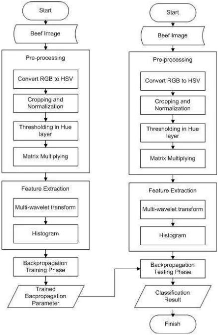
2.1.1 Classification Process by using K-NN and Backpropagation Neural Network
The steps of classification process by using K-NN & Backpropagation Neural Network are shown in figure below:
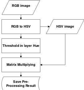
2.2 Experiment Design & Plan 2.2.1 Image Pre-processing
Pre-processing process is the first process in system design. This process is purposed to prepare beef irradiated image before acquiring its feature. By this process, the image will have minimal noise with the optimal condition. The steps of pre-processing process are described below:
- Beef irradiated image will be scaled into 0.2 of its original image.
- After that, the image formatted in .jpeg in the form of digital data 8 bits at each base color RGB (Red, Green, Blue) will be converted into the HSV color space (Hue, Saturation, Value) to see the difference of its brightness. - The next step is thresholding the value of each layer so
that we can get the beef’s position or we can distinguish the beef from the background itself.
- The next step is matrix multiplying from HSV image and the image resulted from thresholding process.
- The last step in pre-processing is save the data result.
Figure II-2 Classification process by using Backpropagation
2.2.2 Image Feature Extraction
Feature extraction is a feature-taking process which describes the characteristic of the image. Feature resulted from feature extraction process is used to compare between one character to another character.
2.2.2.1 Multi-wavelet Transformation
Multi-wavelet Transform used in the process is GHM Multiwavelet. Multi-wavelet can only process a square matrix of pixels and the block size must be multiplying result of 2, whether the data result from pre-processing is not a square matrix. Therefore, in this research, the size of blok result will be normalized into some block size, 32, 64, 128, and 256 size block and rounded to the nearest value. The process is described in picture below:
Figure II-4 Flowchart of multiwavelet process
The next step is multi-wavelet GHM process for each blocks. The GHM basis offers a combination of orthogonality, symmetry, and Compaq support which cannot be achieved bay any other scalar wavelet. Since the GHM filter has two scaling and two wavelet functions, it has two low pass and two high pass sub bands in the transform domain. Due to that, the decomposition of multi-wavelet transformation would appear like picture below:
The highest information is placed in 1st block, which is L1L1. So we get one feature for each small square block. The next step is making an array from all square blocks, and we get the feature of multi-wavelet process.
2.2.2.2 Histogram Feature
The next information to classify beef freshness is its color. The color of a fresh beef is different with the color of a non-fresh beef. Histogram can show the red-color differences. The results from multiwavelet transform are then divided into four kind of feature, they are:
1. The basic feature
2. The basic feature normalized with the total feature 3. The basic feature normalized with the maximum feature 4. The basic feature normalized with the standar deviation. From the process, 16 feature are ready to be the input for classification system as shown in the table below:
Table II-1 Features input for classification system
Feature Size of Block
Basic Feature 32 64 128 256
Basic feature normalized with
the total feature 32 64 128 256
Basic feature normalized with
the maximum feature 32 64 128 256
Basic feature normalized with
the standar deviation 32 64 128 256
2.2.3 Classification Process 2.2.3.1 NN Classification
All parameters resulted from multiwavelet and histogram feature extraction will be used to classify beef freshness. This classification is a process of grouping image into several classes, according to the level of beef freshness classes.
2.2.3.2 Backpropagation Neural Network
Another classification process used in this research is by using backpropagation neural network. All parameters resulted from multiwavelet and histogram feature extraction will be used to classify beef freshness.
Backpropagation neural network has 2 phases:
a)
Training PhaseRGB to HSV
Threshold in layer Hue
Matrix Multiplying RGB image
HSV image
Save Pre-Processing Result
Figure II-3 Flowchart of image pre-processing
Backpropagation learns some kind of patterns to decide which feature will be used in recognition process and classification procedure. The feature value is used to train the backpropagation network. In the training phase, it is needed to set the parameter such as amount of target, amount of hidden layer, activation function, training algotihm and iteration.
b)
Training Recognition PhaseBackpropagation takes a feature and then decides the classification. Modeling is important to make a system simulation to get the output and input of the simulation.
III. SYSTEM ANALYSIS
3.1 Image Pre-processing
Pre-processing process is the first process in system design. This process is purposed to prepare beef irradiated image before acquiring its feature.
Figure III-1 Scaling to 0.2 of the original image
Figure III-2 Convert RGB to HSV color space
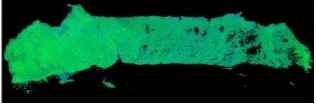
Figure III-3 Thresholding to separate the background and the beef image
Figure III-4 Matrix multiplying process between HSV image and thresholding image
3.2 Image Feature Extraction 3.2.1 Multiwavelet Transformation
Multiwavelet Transform used in the process is GHM Multiwavelet. Multiwavelet can only process a square matrix of pixels and the block size must be multiplying result of 2, whether the data result in from pre-processing is not a square matrix. Therefore, in this research, the size of block result will
be normalized into 4 size of block, that are 32,64,128, and 256 block size and rounded to the nearest value. The picture below describes multiwavelet process:
Figure III-5Input image to multi-wavelet process
Figure III-6Segmented image to small square block size
3.2.2 Histogram Feature
The next information to classify beef freshness is its color. The color of a fresh beef is different with the color of a non-fresh beef. The histogram for 256 size block are shown in figures below:
Figure III-7 Multiwavelet Result
3.3 Classification Process 3.3.1 NN Classification
All parameters resulted from multiwavelet and histogram feature extraction will be used to classify beef freshness. This classification is a process of grouping image into three classes, according to the level of beef freshness classes which are class 1 (fresh beef), class 2 (less fresh beef), and class 3 (non fresh beef). The 1st class or the class for fresh beef is comes from the data feature of day 1, day 2, and day 3. The 2nd class or the less fresh beef class comes from the data feature of day 4 and day 5. The 3rd class or the non fresh beef class comes from the data feature of day 6 and day 7. The accuracy and computation time of NN classification using 16 features are described in table below:
1. List of accuracy from 16 features (in %)
Table III-1 Accuracy from 16 features by using KNN (in %)
From the table above, it can be concluded that the kind of feature doesn’t impact the accuracy, but the block size does give an impact to the accuracy. The best accuracy is given with the block size of 256 with 75%. Therefore, for the next classification system (backpropagation neural network) the 256 block size will be used.
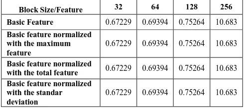
2. List of Computation time from 16 features (in second)
Table III-2 Computation time from 16 features by using KNN (in second)
Block Size/Feature 32 64 128 256
Basic Feature 0.67229 0.69394 0.75264 10.683
Basic feature normalized with the maximum feature
0.67229 0.69394 0.75264 10.683
Basic feature normalized
with the total feature 0.67229 0.69394 0.75264 10.683 Basic feature normalized
with the standar deviation
0.67229 0.69394 0.75264 10.683
From the table above, it can be concluded that the kind of feature doesn’t impact the computation time, but the block size does give an impact. It can be seen also that the bigger the block size, the longer it takes for the system to compute. The fastest computation time is given from 32 block size, which is 0.67229 second.
3.3.2 Backpropagation Classification
In Backpropagation neural network, there are some parameters that define how the system works to process new input. In this research, parameters that being tested are the
Block Size/Feature 32 64 128 256
Basic Feature 71.4286 69.04760 72.619 75
Basic feature normalized with the maximum feature
71.4286 69.04760 72.619 75
Basic feature normalized
with the total feature 71.4286 69.04760 72.619 75 Basic feature normalized
with the standar deviation
71.4286 69.04760 72.619 75
Figure III-9 Histogram value from basic feature of 256 block size
Figure III-10 Histogram value from basic feature normalized with the total feature of
256 block size
Figure III-11 Histogram value from basic feature normalized with the maximum feature
of 256 block size
Figure III-12 Histogram value from basic feature normalized with standard deviation
amount of hidden layer, the amount of learning rate, the amount of neuron in each layer, and the activation function in hidden and output layer. In testing phase, 84 data sets are used as training data, and 112 data sets are used as testing data.
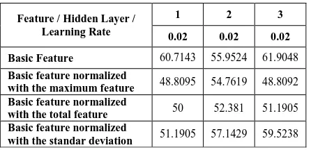
Each network can own more than one hidden layer, even do not own at all. If a network owns some hidden layers, then the last hidden layer will be the one who receive input from input layer. Another parameter called learning rate is used to define the learning rate. The bigger learning rate, then the training process will be done faster. But, if learning rate is too big, the algorithm becomes unstable. This research will observe the impact of the amount of hidden layer and learning rate. The parameter set is error tolerated = 10-10, epoch = 500, activation function = logsig. From the result, the best hidden layer and learning rate can be taken to be the fixed parameters in system. The accuracy result from the test can be seen in the table below:
Table III-3 Accuracy result from various learning rate and amount of hidden layer (in%)
From the table above, it can be seen that learning rate is giving an impact into the accuracy. When learning rate is set into 0.02, it decreased the accuracy. The best accuracy is 71.4286% which is given from learning rate=0.01 and amount of hidden layer=2. The next result is computation time that can be seen from the table below:
Table III-4 Computation time from various learning rate and amount of hidden layer (in second)
From the table, it can be seen that learning rate is giving an impact into the computation time. When learning rate is set into 0.02, the computation time become slower. The fastest computation time is 10.381059 second which is given from learning rate=0.01 and amount of hidden layer=1.
3.4 The False Acceptance Ratio (FAR)
The False Acceptance Ratio (FAR) is defined as the percentage of identification instances in which false acceptance occurs. This can be expressed as a probability. In this research, the false acceptance ratio is 15%, it means that the probability of the system to give the right classification is 85%.
IV. CLOSING
4.1 Conclusions
From the research that has been done, it can be concluded as follows:
1. The use of NN classification gives a better accuracy compare to backpropagation neural network application, 75% with the computation time in 10.683 second, while the best accuracy from using backpropagation is 71.4286% with the computation time 15.800086 second. 2. The best time to keep beef in 7º is for 3 days only, after
that, the beef is not proper to consumed based on the level of red-color-classification.
3. The weakness of this experiment is that by using color anlaysis which come from 32 until 256 size of block of pixels, the decision of beef freshness classification have not able to give the sharp classification.
4. The feature between 1st class and 2nd class is significantly different, the feature between 1st class and 3rd class is significantly different tto. But the feature between the 2nd class and the 3rdclass haven’t been significantly different. 4.2 Advices
From the research that has been done, things that can be suggested are:
1. Color analysis for the next time should be more sensitive. 2. The size of pixels should be bigger to get the more
sensitive system.
3. Try another feature extraction process to improve the feature quality.
4. Try to build a more complex system to classify freshness of beef by using sensor.
V. REFERENCES
The references used in this research are:
1. Chen, K, and friends. (2010). Color Grading of Beef Fat by Using Computer Vision and Support Vector Machine. Computers and Electronics in Agriculture.
2. ElMasry, Gamal, and friends. (2012). Near-Infrared Hyperspectral Imaging for Predicting Colour, pH, a nd Tenderness of Fresh Beef. Journal of Food Engineering. 3. Khosravi, Maziyar, and Mazaheri Amin. (2011). Block
Feature Based Image Fusion Using Multi Wavelet Transform. International Journal of engineering Science and Technology (IJEST)
4. Lasztity, Radomir. Food Quality and Standards – Vol II – Meat and Meat Products. Department of Biochemistry & Food Technology, Budapest University of Technology & Econimic:Hungary
Feature/Hidden Layer/Learning Rate
1 2 3
0.02 0.02 0.02
Basic Feature 30.60872 27.748232 49.5246
Basic feature normalized with the maximum feature
10.751629 16.528081 22.893523
Basic feature normalized with the total feature
10.799773 15.234657 16.390534
Basic feature normalized with the standar deviation
10.908808 13.922928 21.670742
Feature / Hidden Layer / Learning Rate
1 2 3
0.02 0.02 0.02
Basic Feature 60.7143 55.9524 61.9048
Basic feature normalized
with the maximum feature 48.8095 54.7619 48.8092 Basic feature normalized
with the total feature 50 52.381 51.1905
Basic feature normalized