DETERMINING PEAK DISCHARGE FACTOR USING SYNTHETIC
UNIT HYDROGRAPH MODELLING (CASE STUDY: UPPER
KOMERING SOUTH SUMATERA, INDONESIA)
* Rosmalinda Permatasari 1, Dantje Kardana Natakusumah 2 and Arwin Sabar31Faculty of Civil Engineering, Tridinanti University, Indonesia; 2,3Bandung Institute of Technology, Indonesia
*Corresponding Author: Received: 16 June 2016, Revised: 07 August 2016, Accepted: 30 Nov 2016 ABSTRACT: Synthetic unit hydrograph methods are popular and play an important role in many water resources design especially in the analysis of flood discharge of ungagged watersheds. These methods are simple, requiring only watershed characteristics such as area and river length and in some cases it may also include land use characteristics. Therefore, these methods serve as useful tools to simulate runoff from ungagged watersheds and watersheds undergoing land use change. To develop a synthetic unit hydrograph, several techniques are available. Several most popular unit hydrographs methods such as Nakayasu, Snyder-Alexeyev, SCS, and GAMA-1 are popular and commonly used in Indonesia for computing both peak discharge rate and the shape of flood hydrograph. This paper presents a simple approach for determining a consistent dimensionless unit hydrograph based on mass conservation principles. The results for peak discharge in several hydrographs methods are Nakayasu 607.32 m3/sec, SCS 668.62 m3/sec, ITB-1 675.42 m3/sec, ITB-2 642.805 m3/sec in periode time return
2 years.
Key Words: Synthetic Unit Hydrograph (SUH), Flood Hydrograph, Hydrology, Rainfall, Runoff.
1. INTRODUCTION
Unit Hydrograph (UH) is the most popular and widely used method for analyzing and deriving flood hydrograph resulting from a known storm in a basin area. The term ‘Synthetic’ in synthetic unit hydrograph (SUH) denotes the unit hydrograph (UH) derived from watershed characteristics rather than from rainfall-runoff data [1].
The determination of the pick discharge value and the runoff volume of a watershed are crucial in managing natural disasters and designing and constructing water structures. Therefore different methods have been developed. Dimensionless unit hydrograph developed by United States soil conservation service (SCS) provides a shape to the unit hydrograph and therefore leads to more reproducible results than the Snyder method [2]-[3].
The plotting positions of the SCS dimensionless unit hydrograph are expressed as the ratios t/tp and
Q/Qp. tp is the time to peak Qp is the peak discharge.
S-curve hydrograph may be defined as the hydrograph of direct runoff resulting from a continuous effective rainfall of uniform intensity 1/D cm/h [4].
Human activities have always been accompanied by changes in land structure, the destruction of natural resources and urban developments. Cosmopolitan developments on the surface of the watershed will be included in the increase in peak discharge and runoff volume of the watershed [2]-[3]. Upper Komering basin is part of Musi River support operational at South Sumatera and it is located in equatorial region
with the average annual rainfall is 2000 mm [5]. Estimating the maximum flood discharge is necessary for predicting watershed hydrological behavior. Major problems concerning hydrological predictions include a lack or low accuracy of rain data, high cost, lack of information about catchments and the length of time required to obtain study results [2].
The production and behavior of runoff are functions of land use types and changes. The hydrological response of a river basin is based on the relationship between basin geomorphology (catchments area, shape of basin, topography, channel slope, stream density and channel storage) and its hydrology. Many studies have been carried out on the efficiency of artificial unit hydrographs in Indonesia such as study at Citarum Basin and Upper Ciliwung [6]-[7].
2. STUDY AREA
The Upper Komering watershed an area of about 4260 km2. The temperate humid climate 28.40 – 32.20
C, humidity 80% and ratio sunshine 29%. An average annual rainfall 2602.08 mm, wet season during October-May and dry season during June-September [8]. The area's climate is equatorial region and it’s present at Figure 1.
Fig. 1 The location of study area 3. MATERIALS AND METHOD
The study was intended to use methods and models to simulate rainfall-runoff processes in unit hydrograph. In addition, this study attempted to determine the shape and dimensions of outlet runoff hydrographs in a 4260 km2 area in the Upper
Komering Basin, which is located in the South Sumatera Province of Indonesia.
Model Description
SCS Model
The SCS (1957) method computes the runoff
volume (V) and peak discharge (qp) of a triangular
hydrograph, respectively, as follows : V- 𝟏𝟐qpta -
𝟏
𝟐 qp (tp +te) (1) qp = 𝟑
𝟒 V/tp (2)
where qp is peak discharge in mm/h/mm, te is the time
from peak to the tail end of the hydrograph (1.67tp),
and tp is in hours (=1/2T + tL). To determine the SUH
shape from the non-dimensional q/qp versus the t/tp
hydrograph, the time to peak (tp) and peak discharge (qp) are computed as follows :
tp = D/2 + tL (3)
qp = 484A/tp (4)
where D is the duration of rainfall (h), qp is in cfs A
is the area in square miles, tp is in h (base time = 3/8tp),
and tL is the lag time from centroid of rainfall to peak
discharge (qp) (h). The tL can be estimated from
watershed characteristics using curve number CN, watershed length, and slope. With known qp, tp, and
the specified dimensionless UH, an SUH can be derived [1]-[2]-[9]-[10].
Snyder’s Model
Snyder (1938) used three parameters, i.e., lag to
peak tL, peak discharge Qp, and base time tB, to
describe the hydrograph, and these are expressed as : tL = CT(L.LCA)0.03 (5)
Qp = 640.Cp.A/tL (6)
tB = 3 + 3.(tL/24) (7)
where L is the length of the main stream from the outlet to the catchment boundary in miles, LCA is the distance from the outlet to a point on the stream nearest to the centroid of the catchment in miles, CT is a non-dimensional coefficient, A is the area of the catchment in square miles, Cp is another
non-dimensional coefficient, tL, Qp, and tB are in h, ft3/s
(or cfs), and days. The formula hold for rainfall-excess duration TD = tL/5.5. For varying duration, the
lag time is adjusted as: tLR = tL + (T - TD)/4, where tLR
is revised lag time (h) and T is actual TD. Snyder’s
method is applicable to fairly large catchments only, e.g., 100– 500 km2 [1]-[2]-[9]-[10].
SUH ITB Model
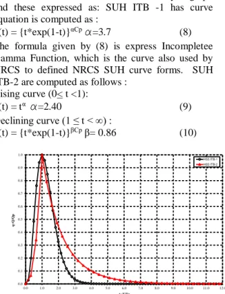
SUH ITB model have two basic method SUH ITB-1 and SUH ITB-2 to describe curve hydrograph and these expressed as: SUH ITB -1 has curve equation is computed as :
q(t) = {t*exp(1-t)}αCp α=3.7 (8) The formula given by (8) is express Incompletee Gamma Function, which is the curve also used by NRCS to defined NRCS SUH curve forms. SUH ITB-2 are computed as follows :
Rising curve (0< t <1):
q(t) = tα α=2.40 (9)
Declining curve (1 ≤ t < ∞) :
q(t) = {t*exp(1-t)}βCp β= 0.86 (10)
Fig. 2 SUH ITB-1 and ITB -2 dimensionless
0.0 0.1 0.2 0.3 0.4 0.5 0.6 0.7 0.8 0.9 1.0 0.0 1.0 2.0 3.0 4.0 5.0 6.0 7.0 8.0 9.0 10.0 11.0 12.0 q= Q /Q p t=T/Tp HSS ITB-1 HSS ITB-2
Figure 2 describe the horizontal axis is t = T/Tp
and the vertical axis q = Q/Qp. Base on SUH
definition and mass conversion principle, it can be inferred the effective rainfall volume in watershed, SUH volume should equal with peak time (Tp) so the
computation peak discharge derived ITB formula [11]-[12]-[13]. The formula respectively as :
Qp = 𝑲𝒑.𝑹.𝑨𝒘 𝑻𝒑 m
3/s (11)
Qp = Peak discharge unit hydrograph m3/s
Kp = 1/(3.6 . ASUH ) = peak rate factor m3/
s/km2/mm
R = Rainfall unit in 1.00 mm Tp = peak time in hour Aw = Watershed area km2
ASUH= Dimensionless unit hydrograph area
Nakayasu Model
The Nakayasu method was developed by applying a dimensionless unit hydrograph based on the Horner and Flynt method for estimating design floods in several small urban watersheds of Japan [9]-[14]-[15]-[16]-[17]-[18]-[19].
4. RESULTS AND DISCUSSIONS
Komering river in upper has a catchment area 4260 km2, effective lenght 180 km. In this study the
rainfall datas undertaken from three rainfall station Banding Agung, Muara Dua and Martapura, then peak discharge data undertaken from Perjaya headwork. Table 1 describes of characteristics study area undertaken. Simulated hydrographs were used to observed hydrographs. The model results for peak discharge (qp) and the time to peak (tp). From listed in
Table 1, were calculated by applying a SUH models and it present in Table 2. Table 3 shows the values of peak discharge. It were computed from rainfall distribution and the values of base flow from dimension unit hydrograph at the first hour 0.034. The peak discharge were computed and the values is 5,131.036 m3/s. In addition, similarities were
observed for the outlet runoff volume parameter in SCS, Snyder, ITB-1 and ITB-2. Triangular and comparisons have proven the difference among UH not significant and it presents in Table 4.
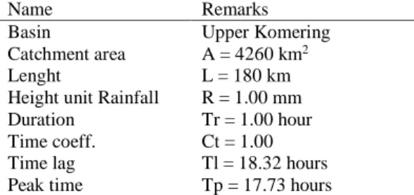
Table 1 Characteristics of Upper Komering area
Name Remarks
Basin
Catchment area Lenght
Height unit Rainfall Duration Time coeff. Time lag Peak time Upper Komering A = 4260 km2 L = 180 km R = 1.00 mm Tr = 1.00 hour Ct = 1.00 Tl = 18.32 hours Tp = 17.73 hours Base time Peak coeff. Alpha SUH area Qp Rainfall volume Tb = 177.3 hours 1.00 2.00 1.3161 50.7 m3/s 4,260,000 m3
Table 4 Peak discharge values in all method
Time return (year )
QT
(m3/s)
Nakayasu SCS ITB-1 ITB-2
2 607,315 668,617 675,420 642,805
5 844,157 977,715 978,548 913,429
10 1045,578 1218,335 1220,946 1128,841
20 1267,438 1481,886 1486,444 1481,886
Table 4 defines the hydrograph dimensions in the study basin using the Snyder, SCS and ITB methods. The results demonstrate that a comparable level of performance was achieved for all methods and it describes in Figure 3. Peak discharge hydrographs were similar and showed negligible errors, but the hydrographs differed more noticeably for peak discharge.
Fig. 3 The hydrograph in the study area
5. CONCLUSION
This study has determined that, compared to other models, to defined the model which is the most efficient model to use in determining peak discharge. The results demonstrate peak discharge hydrographs were similar. The proposed parameter estimations methods are simple to use, and gives accurate results of the actual as verified using simulation and field data.
6. ACKNOWLEDGEMENTS
This paper is part of dissertation research in The Research Division of The Environmental Technology Management-Bandung Institute of Technology (ITB). I wish to thank to The Head of Research Division Prof. Dr. Ir. Arwin Sabar, MS and Dr. Ir. Dantje Kardana Natakusumah as research promotor.
0,0 2,5 5,0 7,5 10,0 12,5 15,0 17,5 20,0 22,5 25,0 27,5 30,0 32,5 35,0 37,5 40,0 0,0 500,0 1.000,0 1.500,0 2.000,0 2.500,0 1 7 13 19 25 31 37 43 49 55 61 67 73 79 85 91 97103109115121127133139145151157 R (m m ) Q (m 3/ s) Infiltration Eff. rainfall Nakayasu (Alpha=2.0) SCS ITB-1 (Exact) ITB-2 (Exact)
Table 2. Dimensionless and dimension unit hydrograph of Upper Komering River
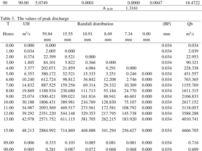
Table 3. The values of peak discharge
T UH Rainfall distribution (BF) Qb Hours m3/s 59.84 15.55 10.91 8.69 7.34 0.00 mm m3/s mm mm mm mm mm mm 0.00 0.000 0.000 0.034 0.034 1.00 0.034 2.005 0.000 0.034 2.039 2.00 0.374 22.399 0.521 0.000 0.034 22.953 3.00 1.405 84.101 5.822 0.366 0.000 0.034 90.321 4.00 3.377 202.071 21.859 4.084 0.291 0.000 0.034 228.338 5.00 6.353 380.172 52.521 15.333 3.251 0.246 0.000 0.034 451.557 6.00 10.240 612.724 98.812 36.842 12.208 2.746 0.000 0.034 763.365 7.00 14.832 887.525 159.256 69.314 29.332 10.309 0.000 0.034 1155.769 8.00 19.869 1188.934 230.680 111.713 55.184 24.770 0.000 0.034 1611.315 9.00 25.074 1500.421 309.021 161.816 88.941 46.601 0.000 0.034 2106.833 10.00 30.188 1806.431 389.981 216.769 128.830 75.107 0.000 0.034 2617.152 11.00 34.987 2093.569 469.517 273.561 172.581 108.792 0.000 0.034 3118.053 12.00 39.292 2351.220 544.148 329.353 217.795 145.738 0.000 0.034 3588.288 13.00 42.978 2571.752 611.115 381.705 262.215 183.920 0.000 0.034 4010.741 15.00 48.213 2884.992 714.869 468.888 341.294 256.627 0.000 0.034 4666.705 89.00 0.006 0.333 0.103 0.085 0.081 0.081 0.000 0.034 0.716 90.00 0.005 0.281 0.087 0.072 0.068 0.068 0.000 0.034 0.609 Peak discharge = 5,131.036 m3/s i T
(hours) Dimensionless unit hydrograph Dimension unit hydrograph
t = T/Tp q = Q/Qp A Q (m3/s) V (m3) (1) (2) (3) (4) (5) (6) 0 0.00 0.0000 0.0000 0.0000 0.0000 0.0000 1 1.00 0.0564 0.0007 0.0000 0.0335 60.3146 2 2.00 0.1128 0.0074 0.0002 0.3743 734.0876 3 3.00 0.1692 0.0277 0.0010 1.4054 3203.5774 4 4.00 0.2256 0.0666 0.0027 3.3769 8608.2457 5 5.00 0.2819 0.1253 0.0054 6.3533 17514.2962 6 6.00 0.3383 0.2020 0.0092 10.2395 29867.0299 7 7.00 0.3947 0.2925 0.0139 14.8319 45128.5658 8 8.00 0.4511 0.3919 0.0193 19.8689 62461.3640 9 9.00 0.5075 0.4946 0.0250 25.0743 80897.7093 10 10.00 0.5639 0.5954 0.0307 30.1882 99472.4853 11 11.00 0.6203 0.6901 0.0362 34.9867 117314.7935 15 15.00 0.8458 0.9510 0.0524 48.2126 169516.7717 89 89.00 5.0185 0.0001 0.0000 0.0056 21.9193 90 90.00 5.0749 0.0001 0.0000 0.0047 18.4722 A SUH 1.3161
7. REFERENCES
[1] Bhunya, P.K., Berndtsson, R., Ojha, Mishra. (2007). Suitability of Gamma, Chi-square, Weibull, and Beta distributions as synthetic unit hydrographs. Journal Hydrology - Elsevier. [2] Khaleghi,M.R.,Gholami, V., Ghodusi,
Hosseini. (2011). Efficiency of the geomorphologic instantaneous unit hydrograph method in flood. Journal of Hydrology. [3] Jena, S.K., Tiwari, K.N. (2006). Modeling
synthetic unit hydrograph parameters with geomorphologic parameters of watersheds.
Journal of Hydrology.
[4] Chow, V. (1964). Handbook of Applied
Hydrology. New York: McGraw-Hill, NY,
USA.
[5] Tjasyono, B. (2004). Klimatologi. Bandung: Penerbit ITB.
[6] Harlan, D. d. (2009). Penentuan Debit Harian Menggunakan Pemodelan Rainfall Runoff GR4J untuk Analisa Unit Hidrograf pada DAS Citarum Hulu. Jurnal Teknik Sipil, Jurnal
Teoretis dan Terapan Bidang Rekayasa Sipil, ITB.
[7] Nugroho, S. (2001). Analisis Hidrograf Satuan Sintetik Metode Snyder, Clark dan SCS dengan Menggunakan Model HEC-1 di DAS Ciliwung Hulu. Jurnal Sains dan Teknologi Modifikasi
Cuaca.
[8] Rusman, A. (2004). Simulasi Alokasi Air pada
Daerah Aliran Sungai Komering Bagian Hulu dalam Pemenuhan Kebutuhan Air Tahun 2020.
Bandung: FTSL-ITB.
[9] Kang, M.S., et.al. (2013). Estimating design floods based on the critical storm duration for small watersheds. Journal of Hydro-Enviroment.
[10] Karmaker,T., Dutta, S. (2010). Generation of synthetic seasonal hydrographs for a large river basin. Journal Hydrology-Elsevier.
[11] Natakusumah D.K., Hatmoko W., and Harlan D. (2011). Prosedure Umum Perhitungan Hidrograf Satuan Sintetis (HSS) dan Contoh Penerapannya Dalam Pengembangan HSS ITB-1 dan HSS ITB-2. Journal Teknik Sipil ITB, Vol.
18 No. 3 .
[12] Natakusumah, D. (2009). Prosedure Umum Penentuan Hidrograf Satuan Sintetis Untuk Perhitungan Hidrograf Banjir Rencana. Seminar
Nasional Sumber Daya Air. Bandung.
[13] Natakusumah, D. (2014). Cara Menghitung
Debit Banjir Dengan Metoda Hidrograf Satuan Sintetis . Bandung: ITB.
[14] Junia, N., dkk. (2015). Kesesuaian Model Hidrograf Satuan Sintetik Studi Kasus Sub Daerah Aliran Sungai Siak Bagian Hulu. Jom
FTEKNIK .
[15] Sihotang, R., dkk. (2011). Analisis Banjir Rancangan dengan Metode HSS Nakayasu pada Bendung Gintung. Universitas Gunadarma . Depok: Proceeding PESAT (Psikologi, Ekonomi, Sastra, Arsitektur dan Sipil, Vol.4 , ISSN:1858-255.
[16] Hadisusanto, N. (2011). Aplikasi Hidrologi. Yogyakarta: Media Utama.
[17] Indarto. (2010). Dasar Teori dan Contoh
Aplikasi Model Hidrologi. Jakarta: Bumi
Aksara.
[18] Kamiana, I. (2012). Teknik Perhitungan Debit
Rencana Bangunan Air. Yogyakarta: Graha
Ilmu.
[19] Limantara, L. (2010). Hidrologi Praktis. Bandung: Lubuk Agung.
Copyright © Int. J. of GEOMATE. All rights reserved, including the making of copies unless permission is obtained from the copyright proprietors.