Linear Circuit Design Handbook
Hank Zumbahlen
with the engineering staff of Analog Devices
AMSTERDAM • BOSTON • HEIDELBERG • LONDON • NEW YORK • OXFORD PARIS • SAN DIEGO • SAN FRANCISCO • SINGAPORE • SYDNEY • TOKYO
Newnes is an imprint of Elsevier
30 Corporate Drive, Suite 400, Burlington, MA 01803, USA Linacre House, Jordan Hill, Oxford OX2 8DP, UK
Copyright © 2008 by Analog Devices. All rights reserved.
No part of this publication may be reproduced, stored in a retrieval system, or transmitted in any form or by any means, electronic, mechanical, photocopying, recording, or otherwise, without the prior written permission of the publisher.
Permissions may be sought directly from Elsevier ’ s Science & Technology Rights Department in Oxford, UK: phone: ( 44) 1865 843830, fax: ( 44) 1865 853333, E-mail: [email protected]. You may also complete your request online via the Elsevier homepage (http://elsevier.com) , by selecting “ Support & Contact ” then “ Copyright and Permission ” and then “ Obtaining Permissions. ”
Recognizing the importance of preserving what has been written, Elsevier prints its books on acid-free paper whenever possible.
Library of Congress Cataloging-in-Publication Data
Linear circuit design handbook / edited by Hank Zumbahlen ; with the engineering staff of Analog Devices.
p. cm.
ISBN 978-0-7506-8703-4
1. Electronic circuits. 2. Analog electronic systems. 3. Operational amplifi ers. I. Zumbahlen, Hank. II. Analog Devices, inc.
TK7867.L57 2008
627.39 5--dc22 2007053012
British Library Cataloguing-in-Publication Data
A catalogue record for this book is available from the British Library.
ISBN: 978-0-7506-8703-4
For information on all Newnes publications visit our Web site at www.books.elsevier.com
Typeset by Charon Tec Ltd (A Macmillan Company), Chennai, India www.charontec.com
Contents
Preface ...ix
Chapter 1: The Op Amp ... 1
Section 1-1: Op Amp Operation ...3
Section 1-2: Op Amp Specifi cations ... 25
Section 1-3: How to Read a Data Sheet ... 69
Section 1-4: Choosing an Op Amp ... 81
Chapter 2: Other Linear Circuits ... 83
Section 2-1: Buffer Amplifi ers ... 85
Section 2-2: Gain Blocks ... 89
Section 2-3: Instrumentation Amplifi ers ... 91
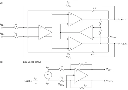
Section 2-4: Differential Amplifi ers ... 107
Section 2-5: Isolation Amplifi ers ... 109
Section 2-6: Digital Isolation Techniques ... 113
Section 2-7: Active Feedback Amplifi ers ... 123
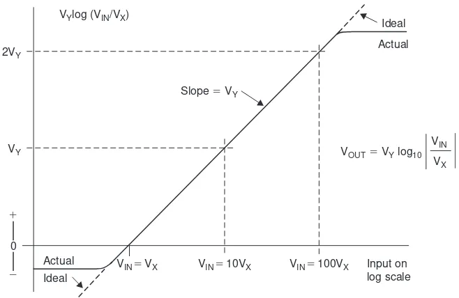
Section 2-8: Logarithmic Amplifi ers ... 125
Section 2-9: High Speed Clamping Amplifi ers ... 131
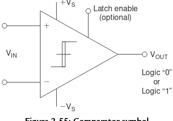
Section 2-10: Comparators ... 137
Section 2-11: Analog Multipliers ... 147
Section 2-12: RMS to DC Converters ... 153
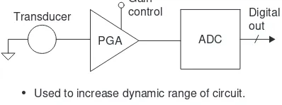
Section 2-13: Programmable Gain Amplifi ers ... 157
Section 2-14: Audio Amplifi ers ... 165
Section 2-15: Auto-Zero Amplifi ers ... 185
Chapter 3: Sensors ... 193
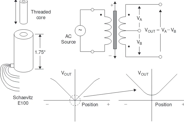
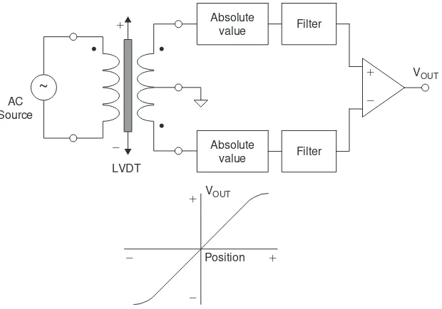
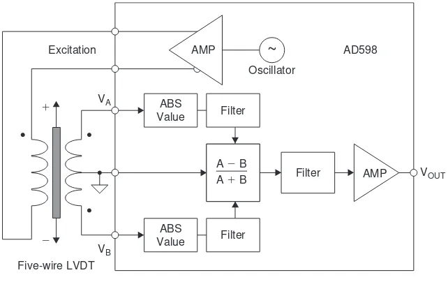
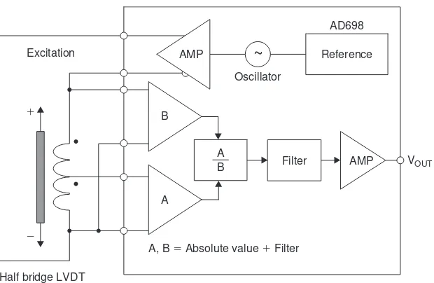
Section 3-1: Positional Sensors ... 195
Section 3-2: Temperature Sensors ... 215
Section 3-3: Charge Coupled Devices ... 241
Chapter 4: RF/IF Circuits ... 245
Section 4-1: Mixers ... 248
Section 4-3: Analog Multipliers ... 257
Section 4-4: Logarithmic Amplifi ers ... 265
Section 4-5: Tru-Power Detectors ... 271
Section 4-6: VGAs ... 275
Section 4-7: Direct Digital Synthesis ... 281
Section 4-8: PLLs ... 289
Chapter 5: Fundamentals of Sampled Data Systems ... 307
Section 5-1: Coding and Quantizing ... 309
Section 5-2: Sampling Theory ... 327
Chapter 6: Converters ... 337
Section 6-1: DAC Architectures ... 340
Section 6-2: ADC Architectures ... 371
Section 6-3: Sigma–Delta Converters ... 407
Section 6-4: Defi ning the Specifi cations ... 431
Section 6-5: DAC and ADC Static Transfer Functions and DC Errors ... 433
Section 6-6: Data Converter AC Errors ... 443
Section 6-7: Timing Specifi cations ... 483
Section 6-8: How to Read a Data Sheet ... 487
Section 6-9: Choosing a Data Converter ... 509
Chapter 7: Data Converter Support Circuits ... 513
Section 7-1: Voltage References ... 515
Section 7-2: Analog Switches and Multiplexers ... 531
Section 7-3: Sample-and-Hold Circuits ... 555
Section 7-4: Clock Generation and Distribution Circuits ... 565
Chapter 8: Analog Filters ... 581
Section 8-1: Introduction ... 583
Section 8-2: The Transfer Function ... 587
Section 8-3: Time Domain Response ... 597
Section 8-4: Standard Responses ... 599
Section 8-5: Frequency Transformations ... 623
Section 8-6: Filter Realizations ... 629
Section 8-7: Practical Problems in Filter Implementation ... 653
Section 8-8: Design Examples ... 663
Chapter 9: Power Management ... 681
Section 9-2: Switch Mode Regulators ... 701
Section 9-3: Switched Capacitor Voltage Converters ... 741
Chapter 10: Passive Components ... 753
Section 10-1: Capacitors ... 755
Section 10-2: Resistors and Potentiometers ... 767
Section 10-3: Inductors ... 775
Chapter 11: Overvoltage Effects on Analog Integrated Circuits ... 779
Section 11-1: Overvoltage Effects ... 781
Section 11-2: Electrostatic Discharge ... 789
Section 11-3: EMI/RFI Considerations ... 799
Chapter 12: Printed Circuit-Board Design Issues ... 821
Section 12-1: Partitioning ... 824
Section 12-2: Traces ... 827
Section 12-3: Grounding ... 863
Section 12-4: Decoupling ... 881
Section 12-5: Thermal Management ... 885
This work is based on the work of many other individuals who have been involved with applications and Analog Devices since the company started in 1965. Much of the material that appears in this work is based on work that has appeared in other forms. My major job function in this case was one of editor. The list of people I would like to credit for doing the pioneering work include: Walt Kester, Walt Jung, Paul Brokaw, James Bryant, Chuck Kitchen, and many other members of Analog Devices technical community. In addition many others contributed to the production of this edition by helping out with the production of this book by providing invaluable assistance by proofreading and providing commentary. I especially want to thank Walt Kester, Bob Marwin, and Judith Douville, who also did the indexing.
Again, many thanks to those involved in this project.
Hank Zumbahlen Senior Staff Applications Engineer
The Op Amp
■ Section 1-1: Op Amp Operation
■ Section 1-2: Op Amp Specifi cations
■ Section 1-3: How to Read a Data Sheet
In this chapter we will discuss the basic operation of the op amp, one of the most common linear design building blocks.
In Section 1-1 the basic operation of the op amp will be discussed. We will concentrate on the op amp from the black box point of view. There are a good many texts that describe the internal workings of an op amp, so in this work a more macro view will be taken. There are a couple of times, however, that we will talk about the insides of the op amp. It is unavoidable.
In Section 1-2 the basic specifi cations will be discussed. Some techniques to compensate for some of the op amps limitations will also be given.
Section 1-3 will discuss how to read a data sheet. The various sections of the data sheet and how to interpret what is written will be discussed.
Section 1-4 will discuss how to select an op amp for a given application.
Introduction
The op amp is one of the basic building blocks of linear design. In its classic form it consists of two input terminals—one of which inverts the phase of the signal, the other preserves the phase—and an output terminal. The standard symbol for the op amp is given in Figure 1-1 . This ignores the power supply terminals, which are obviously required for operation.
Inputs ()
()
Figure 1-1 : Standard op amp symbol
SECTION 1-1
The name “ op amp ” is the standard abbreviation for operational amplifi er. This name comes from the early days of amplifi er design, when the op amp was used in analog computers. (Yes, the fi rst computers were analog in nature, rather than digital.) When the basic amplifi er was used with a few external components, various mathematical “ operations ” could be performed. One of the primary uses of analog computers was during World War II, when they were used for plotting ordinance trajectories.
Voltage Feedback Model
The classic model of the voltage feedback (VFB) op amp incorporates the following characteristics: 1. Infi nite input impedance
2. Infi nite bandwidth 3. Infi nite gain
4. Zero output impedance 5. Zero power consumption
None of these can be actually realized, of course. How close we come to these ideals determines the quality of the op amp.
This is referred to as the VFB model. This type of op amp comprises nearly all op amps below 10 MHz bandwidth and on the order of 90% of those with higher bandwidths ( Figure 1-2 ).
Positive supply
• Ideal op amp attributes – Infinite differential gain
– Zero common mode gain – Zero offset voltage
– Zero bias current
– Infinite bandwidth
• Op amp input attributes – Infinite impedance
– Zero bias current
– Respond to differential voltages
– Do not respond to common mode voltages
• Op amp output attributes – Zero impedance Negative supply
Output Inputs
()
()
Op amp
Figure 1-2 : The attributes of an ideal op amp
Basic Operation
The basic operation of the op amp can be easily summarized. First we assume that there is a portion of the output that is feedback to the inverting terminal to establish the fi xed gain for the amplifi er. This is negative feedback. Any differential voltage across the input terminals of the op amp is multiplied by the amplifi er ’ s open-loop gain. If the magnitude of this differential voltage is more positive on the inverting ( ) terminal than on the non-inverting ( ) terminal, the output will go more negative. If the magnitude of the
set by the feedback. Note from this that the inputs respond to differential-mode not common-mode input voltage:
A R
R FB IN
(1-1)
Inverting and Non-Inverting Confi gurations
There are two basic ways confi gure the VFB op amp as an amplifi er. These are shown in Figure 1-3 and Figure 1-4 .
Figure 1-3 shows what is known as the inverting confi guration. With this circuit, the output is out of phase with the input. The gain of this circuit is determined by the ratio of the resistors used and is given by:
A R
R FB IN
(1-2a) Figure 1-4 shows what is know as the non-inverting confi guration. With this circuit, the output is in phase with the input. The gain of the circuit is also determined by the ratio of the resistors used and is given by:
A R
R FB IN
1 (1-2b)
Note that since the output drives a voltage divider (the gain setting network) the maximum voltage available at the inverting terminal is the full output voltage, which yields a minimum gain of 1.
Also note that in both cases the feedback is from the output to the inverting terminal. This is negative feedback and has many advantages for the designer. These will be discussed in more detail further in this chapter. It should also be noted that the gain is based on the ratio of the resistors, not their actual values. This means that the designer can choose just about any value he or she wishes within practical limits.
If the value of the resistors is too low, a great deal of current would be required from the op amps output for operation. This causes excessive dissipation in the op amp itself, which has many disadvantages. The increased dissipation leads to self-heating of the chip, which could cause a change in the DC characteristics of the op amp itself. Also the heat generated by the dissipation could eventually cause the junction
temperature to rise above the 150 ° C, the commonly accepted maximum limit for most semiconductors.
VIN
VOUT Op amp
RFB
RIN
Summing point
RFB RIN G
VIN VOUT
1
The junction temperature is the temperature at the silicon chip itself. On the other end of the spectrum, if the resistor values are too high, there is an increase in noise and the susceptibility to parasitic capacitances, which could also limit bandwidth and possibly cause instability and oscillation.
From a practical sense, resistors below 10 and above 1 M become increasingly diffi cult to purchase especially if precision resistors are required.
Let us look at the case of an inverting amp in a little more detail. Referring to Figure 1-5 , the non-inverting terminal is connected to ground. (We are assuming a bipolar ( and ) power supply.) Since the op amp
will force the differential voltage across the inputs to zero, the inverting input will also appear to be at ground. In fact, this node is often referred to as a “ virtual ground .”
VIN Op amp
RFB RIN
I1 I2
VOUT
Figure 1-5 : Inverting amplifi er gain
If there is a voltage (V IN ) applied to the input resistor, it will set up a current (I1) through the resistor (R IN ) so that:
I V
R IN IN
1 (1-3)
VIN VOUT
Op amp
RFB
RIN
R
FB RIN G
VIN VOUT
1
Since the input impedance of the op amp is infi nite, no current will fl ow into the inverting input. Therefore, this same current (I1) must fl ow through the feedback resistor (R FB ). Since the amplifi er will force the inverting terminal to ground, the output will assume a voltage (V OUT ) such that:
VOUTI1 RFB (1-4)
Doing a little simple arithmetic we then can come to the conclusion of Eq. (1-1): V
V A
R R OUT
IN
FB IN
(1-5)
Now we examine the non-inverting case in more detail. Referring to Figure 1-6 , the input voltage is applied to the non-inverting terminal. The output voltage drives a voltage divider consisting of R FB and R IN . The name “ R IN ,” in this instance, is somewhat misleading since the resistor is not technically connected to the input, but we keep the same designation since it matches the inverting confi guration, has become a de facto standard, anyway. The voltage at the inverting terminal (V a ), which is at the junction of the two resistors, is:
V R
R R V
a IN
IN FB OUT
(1-6)
The negative feedback action of the op amp will force the differential voltage to 0 so:
VaVIN (1-7)
Again applying a little simple arithmetic we end up with: V
V
R R
R
R R OUT
IN
FB IN IN
FB IN
1 (1-8)
Which is what we specifi ed in Eq. (1-2).
RFB RIN G
VIN VOUT
1
VIN I VOUT
RFB
RIN
Figure 1-6 : Non-inverting amplifi er gain
Open-Loop Gain
The open-loop gain (usually referred to as A VOL ) is the gain of the amplifi er without the feedback loop being closed, hence the name “ open loop .” For a precision op amp this gain can be vary high, on the order of 160 dB or more. This is a gain of 100 million. This gain is fl at from DC to what is referred to as the dominant pole. From there it falls off at 6 dB/octave or 20 dB/decade. (An octave is a doubling in frequency and a decade is 10 in frequency.) This is referred to as a single pole response. It will continue to fall at
this rate until it hits another pole in the response. This second pole will double the rate at which the open-loop gain falls, i.e., to 12 dB/octave or 40 dB/decade. If the open-open-loop gain has dropped below 0 dB (unity gain) before it hits the second pole, the op amp will be unconditionally stable at any gain. This will be typically referred to as unity gain stable on the data sheet. If the second pole is reached while the loop gain is greater than 1 (0 dB), then the amplifi er may not be stable under some conditions ( Figure 1-7 ).
Open-loop gain (dB)
Open-loop gain
(dB) 6 dB/Octave
6 dB/Octave
12 dB/ Octave
Single pole response Two pole response
Figure 1-7 : Open-loop gain (Bode plot)
It is important to understand the differences between open-loop gain, closed-loop gain, loop gain, signal gain, and noise gain ( Figures 1-8 and 1-9 ). They are similar in nature, interrelated, but different. We will discuss them all in detail.
Gain (dB)
log f fCL
Open-loop gain Loop gain
Closed-loop gain Noise gain
Figure 1-8 : Gain defi nition
-• Voltage noise and offset voltage of the op amp are reflected to the output by the noise gain.
• Noise gain, not signal gain, is relevant in assessing stability. • Circuit C has unchanged signal gain, but higher noise gain, thus better stability, worse noise, and higher output offset voltage.
In addition, the open-loop gain can change due to output voltage levels and loading. There is also some dependency on temperature. In general, these effects are of a very minor degree and can, in most cases, be ignored. In fact this nonlinearity is not always included in the data sheet for the part.
Gain-Bandwidth Product
The open-loop gain falls at 6 dB/octave. This means that if we double the frequency, the gain falls to half of what it was. Conversely, if the frequency is halved, the open-loop gain will double, as shown in Figure 1-8 . This gives rise to what is known as the Gain-Bandwidth Product. If we multiply the open-loop gain by the frequency, the product is always a constant. The caveat for this is that we have to be in the part of the curve that is falling at 6 dB/octave. This gives us a convenient fi gure of merit with which to determine if a particular op amp is useable in a particular application ( Figure 1-10 ).
For example, if we have an application with which we require a gain of 10 and a bandwidth of 100 kHz, we require an op amp with, at least, a gain-bandwidth product of 1 MHz. This is a slight oversimplifi cation. Because of the variability of the gain-bandwidth product, and the fact that at the location where the closed-loop gain intersects the open-loop gain the response is actually down 3 dB, a little margin should be included. In the application described above, an op amp with a gain-bandwidth product of 1 MHz would be marginal. A safety factor of at least 5 would be better insurance that the expected performance is achieved.
Stability Criteria
X Y fCL
log f fCL
Y 1 R2
R1 Noise gain Y Gain
(dB) Open-loop gain, A(s)
if gain bandwidth product X then Y fCL X
where fCL Closed-loop bandwidth
Figure 1-10 : Gain-bandwidth product
The question could be then, why would you want an amplifi er that is not unity gain stable. The answer is that for a given amplifi er, the bandwidth can be increased if the amplifi er is not unity gain stable. This is sometimes referred to as decompensated, but the gain criteria must be met. This criteria is that the closed-loop gain must intercept the open-loop gain at a slope of 6 dB/octave (single pole response). If not, the amplifi er will oscillate.
As an example, compare the open-loop gain graphs in Figures 1-11, 1-12, 1-13 . The three parts shown, the AD847, AD848, and AD849, are basically the same part. The AD847 is unity gain stable. The AD848 is stable for gains of two or more. The AD849 is stable for a gain of 10 or more.
100 100
80
60
40
20
0 80
60
40
Open-loop gain (dB)
Phase margin (degrees)
20
100 1 k 10 k 100 k 1 M 10 M 100 M
Frequency (Hz) 0
20
15 V Supplies 1 k Load
5 V Supplies 500 Load
Phase Margin
One measure of stability is phase margin. Just as the amplitude response does not stay fl at and then change instantaneously, the phase will also change gradually, starting as much as a decade back from the corner frequency. Phase margin is the amount of phase shift that is left until you hit 180 ° measured at the unity gain point.
The manifestation of low phase margin is an increase in the peaking of the output just before the close loop gain intersects the open-loop gain (see Figure 1-14 ).
100 100
80
60
40
20
0 80
60
40
Open-loop gain (dB)
Phase margin (degrees)
20
100 1 k 10 k 100 k 1 M 10 M 100 M
Frequency (Hz) 0
20
15 V Supplies 1 k Load
5 V Supplies 500 Load
Figure 1-12 : AD848 open-loop gain
120 100
80
60
40
20
0 100
80
60
Open-loop gain (dB)
Phase margin (degrees)
40
100 1 k 10 k 100 k 1M 10 M 100 M
Frequency (Hz) 20
0
15 V Supplies 1 k Load
5 V Supplies 500 Load
Closed-Loop Gain
This, of course, is the gain of the amplifi er with the feedback loop closed, as opposed the open-loop gain, which is the gain with the feedback loop opened. It has two forms, signal gain and noise gain. These are described and differentiated below.
The expression for the gain of a closed-loop amplifi er involves the open-loop gain. If G is the actual gain, N G is the noise gain (see below), and A VOL is the open-loop gain of the amplifi er, then:
From this you can see that if the open-loop gain is very high, which it typically is, the closed-loop gain of the circuit is simply the noise gain.
Signal Gain
This is the gain applied to the input signal, with the feedback loop connected. In the basic operation section above, when we talked about the gain of the inverting and non-inverting circuits, we were actually more correctly talking about the closed-loop signal gain. It can be inverting or non-inverting. It can even be less than unity for the inverting case. Signal gain is the gain that we are primarily interested in when designing circuits. The signal gain for an inverting amplifi er stage is:
A R
R FB
IN (1-10)
and for a non-inverting amplifi er it is:
Noise Gain
Noise gain is the gain applied to a noise source in series with an op amp input. It is also the gain applied to an offset voltage. The noise gain is equal to:
A R
R FB IN
1 (1-12)
Noise gain is equal to the signal gain of a inverting amp. It is the same for either an inverting or non-inverting stage.
It is the noise gain that is used to determine stability. It is also the closed-loop gain that is used in Bode plots. Remember that even though we used resistances in the equation for noise gain, they are actually impedances (see Figure 1-9 ).
Loop Gain
The difference between the open- and the closed-loop gain is known as the loop gain. This is useful information because it gives you the amount of negative feedback that can apply to the amplifi er system (see Figure 1-8 ).
Bode Plot
The plotting of open-loop gain versus frequency on a log–log scale gives is what is known as a Bode (pronounced boh dee ) plot. It is one of the primary tools in evaluating whether a particular op amp is
suitable for a particular application.
If you plot the open-loop gain and then the noise gain on a Bode plot, the point where they intersect will determine the maximum closed-loop bandwidth of the amplifi er system. This is commonly referred to as the closed-loop frequency (F CL ). Remember that the true response at the intersection is actually 3 dB down. One octave above and one octave below F CL , the difference between the asymptotic response and the real response will be less than 1 dB ( Figure 1-15 ).
Open-loop gain Noise gain
fCL 40
30
20
10
10 MHz 3.0 MHz
1.0 MHz 300 KHz
100 KHz 30 KHz
10 KHz 0
Frequency
Gain
The Bode plot is also useful in determining stability. As stated above, if the closed-loop gain (noise gain) intersects the open-loop gain at a slope of greater than 6 dB/octave (20 dB/decade), the amplifi er may be unstable (depending on the phase margin).
Current Feedback Model
There is a type of amplifi ers that have several advantages over the standard VFB amplifi er at high fre-quencies. They are called current feedback (CFB) or sometimes transimpedance amps. There is a possible point of confusion since the currenttovoltage (I/V) converters commonly found in photo -diode applications are also referred to as transimpedance amps. Schematically CFB op amps look similar to standard VFB amps, but there are several key differences.
The input structure of the CFB is different from the VFB. While we are trying not to get into the internal structures of the op amps, in this case a simple diagram is in order (see Figure 1-16 ). The mechanism of feedback is also different, hence the names. But again, the exact mechanism is beyond what we want to cover here. In most cases if the differences are noted, and the attendant limitations observed, the basic operation of both types of amplifi ers can be thought of as the same. The gain equations are the same as for a VFB amp, with an important limitation as noted in the next section.
v
A(s) v
A(s) Open-loop gain VOUT A(s)*v VIN
i
T(s) i T(s)
RO
i
1
R2 R1
VIN
VOUT 1
VOUT
R2 R1
i
T(s) Transimpedance open-loop gain VOUT T(s)*i
~
Figure 1-16 : VFB and CFB amplifi ers
Difference from VFB
One primary difference between the CFB and VFB amps is that there is not a gain-bandwidth product. While there is a change in bandwidth with gain, it is not even close to the 6 dB/octave that we see with VFB (see Figure 1-17 ). Also, a major limitation is that the value of the feedback resistor determines the bandwidth, working with the internal capacitance of the op amp. For every CFB op amp there is a recommended value of feedback resistor for maximum bandwidth. If you increase the value of the resistor, reduce the bandwidth. If you use a lower value of resistor, the phase margin is reduced and the amplifi er could become unstable. This optimum value of resistor is different for different operational conditions. For instance, the value will change for different packages, e.g., SOIC versus DIP (see Figure 1-18 ).
Also, a CFB amplifi er should not have a capacitor in the feedback loop. If a capacitor is used in the
Gain
(dB) G1
G2
G1f1
G2f2f1 f2 log f
Feedback resistor fixed for optimum performance. Larger values reduce bandwidth; smaller values may cause instability. For fixed feedback resistor, changing gain has little effect on bandwidth.
Current feedback op amps do not have a fixed gain-bandwidth product.
Figure 1-17 : CFB amplifi er frequency response
oscillate. You need to be careful of stray capacitances around the inverting input of the op amp for the same reason.
A common error in using a CFB op amp is to short the inverting input directly to the output in an attempt to build a unity gain voltage follower (buffer). This circuit will oscillate. Obviously, in this case, the feedback resistor value will be less than the recommended value. The circuit is perfectly stable if the recommended feedback resistor of the correct value is used in place of the short.
Another difference between the VFB and CFB amplifi ers is that the inverting input of the CFB amp is low impedance. By low we mean typically 50–100 . Therefore, there is not the inherent balance between the inputs that the VFB circuit shows.
Slew-rate performance is also enhanced by the CFB topology. The current that is available to charge the internal compensation capacitor is dynamic. It is not limited to any fi xed value as is often the case in VFB topologies. With a step input or overload condition, the current is increased (current-on-demand) until the overdriven condition is removed. The basic CFB amplifi er has no fundamental slew-rate limit. Limits only come about from parasitic internal capacitances and many strides have been made to reduce their effects.
AD8001AN (PDIP) AD8001AR (SOIC) AD8001ART (SOT-23-5) Gain Gain Gain
Component ⴚ1 ⴙ1 ⴙ2 ⴙ10 ⴙ100 ⴚ1 ⴙ1 ⴙ2 ⴙ10 ⴙ100 ⴚ1 ⴙ1 ⴙ2 ⴙ10 ⴙ100
RF() 649 1050 750 470 1000 604 953 681 470 1000 845 1000 768 470 1000 RG() 649 750 51 10 604 681 51 10 845 768 51 10 RO(Nominal) () 49.9 49.9 49.9 49.9 49.9 49.9 49.9 49.9 49.9 49.9 49.9 49.9 49.9 49.9 RS() 0 0 0
RT(Nominal) () 54.9 49.9 49.9 49.9 49.9 54.9 49.9 49.9 49.9 49.9 54.9 49.9 49.9 49.9 49.9 Small signal
BW (MHz) 340 880 460 260 20 370 710 440 260 20 240 795 380 260 20 0.1 dB Flatness
(MHz) 105 70 105 130 100 120 110 300 145
The combination of higher bandwidths and slew rate allows CFB devices to have good distortion performance while doing so at a lower power.
The distortion of an amplifi er is impacted by the open-loop distortion of the amplifi er and the loop gain of the closed-loop circuit. The amount of open-loop distortion contributed by a CFB amplifi er is small due to the basic symmetry of the internal topology. Speed is the other main contributor to distortion. In most confi gurations, a CFB amplifi er has a greater bandwidth than its VFB counterpart. So at a given signal frequency, the faster part has greater loop gain and therefore lower distortion.
How to Choose Between CFB and VFB
The application advantages of CFB and VFB differ. In many applications, the differences between CFB and VFB are not readily apparent. Today ’ s CFB and VFB amplifi ers have comparable performance, but there are certain unique advantages associated with each topology. VFB allows freedom of choice of the feedback resistor (or impedance) at the expense of sacrifi cing bandwidth for gain. CFB maintains high bandwidth over a wide range of gains at the cost of limiting the choices in the feedback impedance. In general, VFB amplifi ers offer:
● Lower noise
● Better DC performance
● Feedback component freedom
while CFB amplifi ers offer:
● Faster slew rates
● Lower distortion
● Feedback component restrictions
Supply Voltages
Historically the supply voltage for op amps was typically 15 V. The operational input and output range was on the order of 10 V. But there was no hard requirement for these levels. Typically the maximum supply was 18 V. The lower limit was set by the internal structures. You could typically go within 1.5 or 2 V of either supply rail, so you could reasonably go down to 8 V supplies or so and still have a reasonable dynamic range.
Lately though, there has been a trend toward lower supply voltages. This has happened for a couple of reasons.
First, high speed circuits typically have a lower full-scale range. The principal reason for this is the amplifi er’s ability to swing large voltages. All amplifi ers have a slew-rate limit, which is expressed as so many volts per microsecond. So if you want to go faster, your voltage range must be reduced, all other things being equal. Another reason is that to limit the effects of stray capacitance on the circuits, you need to reduce their impedance levels. Driving lower impedances increases the demands on the output stage, and on the power dissipation abilities of the amplifi er package. Lower voltage swings require lower currents to be supplied, thereby lowering the dissipation of the package.
speed op amps typically have breakdown voltage of 7 V, and so the supplies are typically 5 V, or even
lower.
In some cases, operation on batteries established a requirement for lower supply voltages. Lower supplies would then lessen the number of batteries, which, in turn, reduced the size, weight, and cost of the end product.
At the same time there was a movement towards single supply systems. Instead of the typical plus and minus supplies, the op amps operate on a single positive supply and ground, the ground then becoming the negative supply.
Single Supply Considerations
There is nothing in the circuitry of the op amp that requires ground. In fact, instead of a bipolar ( and )
supply of 15 V you could just as easily use a single supply of 30 V (ground being the negative supply), as
long as the rest of the circuit was biased correctly so that the signal was within the common-mode range of op amp. Or, for that matter, the supply could just as easily be 30 V (ground being the most positive supply).
When you combine the single supply operation with reduced supply voltages, you can run into problems. The standard topology for op amps uses a NPN differential pair (see Figure 1-19 ) for the input and emitter followers (see Figure 1-22 ) for the output stage. Neither of these circuits will let you run “ rail-to-rail ” , i.e., from one supply to the other. Some circuit modifi cations are required.
VIN
Figure 1-19 : Standard input stage (differential pair)
The fi rst of these modifi cations was the use of a PNP differential input (see Figure 1-20 ). One of the fi rst examples of this input confi guration was the LM324. This confi guration allowed the input to get close to the negative rail (ground). It could not, however, go to the positive rail, But in many systems, especially mixed signal systems that were predominately digital, this was enough. In terms of precision, the 324 is not a stellar performer.
The NPN input cannot swing to ground. The PNP input cannot swing to the positive rail. The next
modifi cation was to use a dual input. Here a NPN differential pair is combined with a PNP differential pair (see Figure 1-21 ). Over most of the common-mode range of the input both pairs are active. As one rail or the other is approached, one of the inputs turns off. The NPN pair swings to the upper rail and the PNP pair swings to the lower rail.
Another difference is the output stage. The standard output stage, which is a complimentary emitter follower (common collector) confi guration, is typically replaced by a common emitter circuit ( Figure 1-22 ). This allows the output to swing close to the rails. The exact level is set by the V CEsat of the output transistors, which is, in turn, dependent on the output current levels. The only real disadvantage to this arrangement is that the output impedance of the common emitter circuit is higher than the common collector circuit. Most of the time this is not really an issue, since negative feedback reduces the output impedance proportional to the amount of loop gain. Where it becomes an issue is that as the loop gain falls this higher output impedance is more susceptible to the effects of capacitive loading.
VS
VS
Figure 1-20 : PNP input stage
VS
VS
VS
Emitter follower Common emitter
VS
VS VS
Output Output
Figure 1-22 : Output stages: Emitter follower for standard confi guration and common emitter for “ rail-to-rail ” confi guration
Circuit Design Considerations for Single Supply Systems
Many waveforms are bipolar in nature. This means that the signal naturally swings around the reference level, which is typically ground. This obviously will not work in a single supply environment. What is required is to AC couple the signals.
AC coupling is simply applying a high pass fi lter and establishing a new reference level typically
somewhere around the center of the supply voltage range (see Figure 1-23 ). The series capacitor will block the DC component of the input signal. The corner frequency (the frequency at which the response is 3 dB down from the midband level) is determined by the value of the components:
f
R C
c
EQ
1
2 (1-13)
where:
R R R
R R
EQ 4 5 4 5
(1-14)
It should be noted that if multiple sections are AC coupled, each section will be 3 dB down at the corner frequency. So if there are two sections with the same corner frequency, the total response will be 6 dB down; three sections would be 9 dB down, etc. This should be taken into account so that the overall response of the system will be adequate. Also keep in mind that the amplitude response starts to roll off a decade, or more, from the corner frequency.
In an amplifi er circuit such as that of Figure 1-23 , the output bias point will be equal to the DC bias as applied to the op amp ’ s () input. For a symmetric (50% duty cycle) waveform of a 2 Vp-p output level, the
output signal will swing symmetrically about the bias point, or nominally 2.5 1 V (using the values give
In Figure 1-24 (A), an example of a 50% duty cycle square wave of about 2 Vp-p level is shown, with the signal swing biased symmetrically between the upper and lower clip points of a 5 V supply amplifi er. This amplifi er, for example, (an AD817 biased similarly to Figure 1-23 ) can only swing to the limited DC levels as marked, about 1 V from either rail. In cases (B) and (C), the duty cycle of the input waveform is adjusted to both low and high duty cycle extremes while maintaining the same peak-to-peak input level . At the
amplifi er output, the waveform is seen to clip either negative or positive, in (B) and (C), respectively.
Rail-to-Rail
When the input and/or the output can swing very close to the supply rails, it is referred to as “ rail-to-rail. ” There is no industry standard defi nition for this. At Analog Devices (ADI) we have defi ned this at swinging to within 100 mV of either rail. For the output this is driving a standard load, since the actual maximum output level will depend on the output current. Note that not all amplifi ers that are touted as single supply are rail-to-rail. And not all rail-to-rail amplifi ers are rail-to-rail on input and output. It could be one or the other, both, or neither. The bottom line is that you must read the data sheet. In no case can the output actually swing completely to the rails.
Phase Reversal
There is an interesting phenomenon that can occur when the common-mode range of the op amp is exceeded. Some internal nodes can turn off and the output will be pulled to the opposite rail until the input comes back into the operational range (see Figure 1-25 ). Many modern designs take steps to eliminate this problem. Many times this is called out in the bullets on the cover page. Phase reversal is most common when the amplifi er is in the follower mode.
Input Output
Vertical scale: 5 V / division Horizontal scale: 100 s / division
5 V 100 s 5 V 100 s
Figure 1-25 : Phase reversal
Low Power and Micropower
Along with the trend toward single supplies is the trend toward lower quiescent power. This is the power used by the amp itself. We have arrived at the point where there are whole amplifi ers that can operate on the bias current of the 741.
However, low power involves some tradeoffs.
Another approach to lower power is to lower the standing current of the input stage. The result of this is to reduce the bandwidth and to increase the noise.
While the term “ low power ” can mean vastly different things depending on the application, at ADI we have set a defi nition for op amps. Low power means the quiescent current is less than 1 mA per amplifi er. Micropower is defi ned as having a quiescent current less than 100 A per amplifi er. As was the case with “ rail-to-rail, ” this is not an industry wide defi nition.
Processes
The vast majority of modern op amps are built using bipolar transistors.
Occasionally a junction FET is used for the input stage. This is commonly referred to as a Bi-Fet (for Bi polar- FET ). This is typically done to increase the input impedance of the op amp, or conversely, to lower the input bias currents. The FET devices are typically used only in the input stage. For single supply applications, the FETs can be either N-channel or P-channel. This allows input ranges extending to the negative rail and positive rail, respectively.
Complementary-MOS processing (CMOS) is also used for op amps. While historically CMOS has not been that attractive a process for linear amplifi ers, process and circuit design make progressed to the point that quite reasonable performance can be obtained from CMOS op amps.
One particularly attractive aspect of using CMOS is that it lends itself easily to mixed mode (analog and digital) applications. Some examples of this are the DigiTrim and chopper stabilized op amps.
“ DigiTrim ” is a technique that allows the offset voltage of op amps to be adjusted out at fi nal test. This replaces the more common techniques of zener zapping or laser trimming, which must be done at the wafer level. The problem with trimming at the wafer level is that there are certain shifts in parameters due to packaging, etc. that take place after the trimming is done. While the shift in parameters is fairly well understood and some of the shift can be anticipated, trimming at fi nal test is a very attractive alternative. The DigiTrim amplifi ers basically incorporate a small digital-to-analog converter (DAC) used to adjust the offset. Chopper stabilized amplifi ers use techniques to adjust out the offset continuously. This is accomplished by using a DC precision amp to adjust the offset of a wider bandwidth amp. The DC precision amp is switched between a reference node (usually ground) and the input. This then is used to adjust the offset of the “ main ” amp.
DigiTrim and chopper stabilized amplifi ers are covered in more detail in Chapter 2.
Effects of Overdrive on Op Amp Inputs
There are several important points to be considered about the effects of overdrive on op amp inputs. The fi rst is, obviously, damage. The data sheet of an op amp will give “ absolute maximum ” input ratings for the device. These are typically expressed in terms of the supply voltage, but, unless the data sheet expressly says otherwise, maximum ratings apply only when the supplies are present, and the input voltages should be held near zero in the absence of supplies.
A common type of rating expresses the maximum input voltage in terms of the supply, Vss 0.3 V. In effect, neither input may go more than 0.3 V outside the supply rails, whether they are on or off. If current is limited to 5 mA or less, it generally does not matter if inputs do go outside 0.3 V when the supply is off
(provided that no base–emitter reverse breakdown occurs). Problems may arise if the input is outside this range when the supplies are turned on as this can turn on parasitic silicon controlled rectifi ers (SCRs) in the device structure and destroy it within microseconds. This condition is called latch-up , and is much more
to latch-up, avoid the possibility of signals appearing before supplies are established. (When signals come from other circuitry using the same supply there is rarely, if ever, a problem.) Fortunately, most modern integrated circuit (IC) op amps are relatively insensitive to latch-up.
Input stage damage will be limited if the input current is limited. The standard rule-of-thumb is to limit the current to 5 mA. Reverse bias junction breakdown should be avoided at all cost. Note that the common—and differential—mode specifi cations may be different. Also, not all overvoltage damage is catastrophic. Small degradation of some of the specifi cations can occur with constant abuse by overvoltaging the op amp. A common method of keeping the signal within the supplies is to clamp the signal to the supplies with Schottky diodes as shown in Figure 1-26 . This does not, in fact, limit the signal to 0.3 V at all temperatures, but if the Schottky diodes are at the same temperature as the op amp, they will limit the voltage to a safe level, even if they do not limit it at all times to within the data sheet rating. This is easily accomplished if overvoltage is only possible at turn-on, and diodes and op amp will always be at the same temperature then. If the op amp may still be warm when it is repowered, however, steps must be taken to ensure that diodes and op amp are at the same temperature when this occurs.
VS
VS RS
Figure 1-26 : Input overvoltage protection
Many op amps have limited common-mode or differential input voltage ratings. Limits on common-mode are usually due to complex structures in very fast op amps and vary from device to device. Limits on differential input avoid a damaging reverse breakdown of the input transistors (especially super-beta transistors). This damage can occur even at very low current levels. Limits on differential inputs may also be needed to prevent internal protective circuitry from overheating at high current levels when it is conducting to prevent breakdowns—in this case, a few hundred microseconds of overvoltage may do no harm. One should never exceed any “ absolute maximum ” rating, but engineers should understand the reasons for the rating so that they can make realistic assessments of the risk of permanent damage should the unexpected occur.
If an op amp is overdriven within its ratings, no permanent damage should occur, but some of the internal
Introduction
In this section, we will discuss basic op amp specifi cations. The importance of any of these specifi cations depends, of course, on the application. For instance, offset voltage, offset voltage drift, and open-loop gain (DC specifi cations) are very critical in precision sensor signal conditioning circuits, but may not be as important in high speed applications where bandwidth, slew rate, and distortion (AC specifi cations) are typically the key specifi cations.
Most op amp specifi cations are largely topology independent. However, although VFB and CFB op amps have similar error terms and specifi cations, the application of each part warrants discussing some of the specifi cations separately. In the following discussions, this will be done where signifi cant differences exist. It should be noted that not all of these specifi cations will necessarily appear on all data sheets. As the performance of the op amp increases, the more specifi cations it has and the tighter the specifi cations become. Also keep in mind the difference between typical and min/max. At ADI, a specifi cation that is min/max is guaranteed by test. Typical specifi cations are generally not tested.
DC Specifi cations
Open-Loop GainThe open-loop gain is the gain of the amplifi er when the feedback loop is not closed. It is generally measured, however, with the feedback loop closed, although at a very large gain. In an ideal op amp, it is infi nite with infi nite bandwidth. In practice, it is very large (up to 160 dB) at DC. At some frequency (the dominant pole) it starts to fall at 6 dB/octave or 20 dB/decade. (An octave is a doubling in frequency and a decade is 10 in frequency.) This is referred to as a single pole response. The dominant pole frequency will range from in the neighborhood of 10 Hz for some high precision amps to several kHz for some high speed amps. It will continue to fall at this rate until it reaches another pole in the response. This second pole will double the rate at which the open-loop gain falls, that is to 12 dB/octave or 40 dB/decade. If the open-loop gain has gone below 0 dB (unity gain) before the amp hits the second pole, the op amp will be unconditionally stable at any gain. This will be referred to as unity gain stable on the data sheet. If the second pole is reached while the loop gain is greater than 1 (0 dB), then the amplifi er may not be stable under some conditions ( Figure 1-27 ).
Since the open-loop gain falls by half with a doubling of frequency with a single pole response, there is what is called a constant gain-bandwidth product. At any point along the curve, if the frequency is multiplied by the gain at that frequency, the product is a constant. For example, if an amplifi er has a 1 MHz gain-bandwidth product, the open-loop gain will be 10 (20 dB) at 100 kHz, 100 (40 dB) at 10 kHz, etc. This is readily apparent on a Bode plot, which plots gain versus frequency on a log–log scale.
Since a VFB op amp operates as a voltage in/voltage out device, its open-loop gain is a dimensionless ratio, so no unit is necessary. Data sheets sometimes express gain in V/mV or V/ V instead of V/V, for the convenience of using smaller numbers. Or voltage gain can also be expressed in dB terms, as gain in dB = 20 log A VOL . Thus an open-loop gain of 1 V/ V (or 1000 V/mV or 1,000,000 V/V) is equivalent to 120 dB, and so on ( Figure 1-28 ).
For very high precision work, the nonlinearity of the open-loop gain must be considered. Changes in the output voltage level and output loading are the most common causes of changes in the open-loop gain of op amps. A change in open-loop gain with signal level produces a nonlinearity in the closed-loop gain transfer
function, which cannot be removed during system calibration. Most op amps have fi xed loads, so A VOL changes with load are not generally important. However, the sensitivity of A VOL to output signal level may increase for higher load currents (see Figure 1-29).
The severity of this nonlinearity varies widely from one device type to another, and generally is not specifi ed on the data sheet. The minimum A VOL is always specifi ed, and choosing an op amp with a high A VOL will minimize the probability of gain nonlinearity errors. There is no way to compensate for A VOL nonlinearity.
Open-Loop Transresistance of a CFB Op Amp
For CFB amplifi ers, the open-loop response is voltage out for a current in, so it is a transresistance
(expressed in ohms) rather than a gain. This is generally referred to as a transimpedance , since there is an
AC component as well as a DC term. The transimpedance of a CFB amp will usually be in the range of
500 k to 1 M .
A CFB op amp open-loop transimpedance does not vary in the same way as a VFB open-loop gain. Therefore, a CFB op amp will not have the same gain-bandwidth product as in VFB amps. While there is
Gain (dB)
log f fCL
X Y fCL
Y 1 R2 R1 Noise gain Y
Open-loop gain, A(s) if gain bandwidth product X then Y fCL X
where fCL Closed-loop bandwidth
Figure 1-28 : Bode plot (for VFB amps)
Open-loop gain (dB)
Open-loop gain
(dB) 6 dB/Octave
6 dB/Octave
12 dB/ Octave
Single pole response Two pole response
some variation of frequency response with frequency with a CFB amp, it is nowhere near 6 dB/octave (see Figure 1-30) .
VY 50 mV/division
0
–10 V 10 V
Closed-loop gain nonlinearity NG0.07 ppm Open-loop gain nonlinearity 0.07 ppm AVOL,Max 9.1 million, AVOL,Min 5.7 million AVOL (average) 8 million
VX Output voltage VOS
(0.5 V/division)
(RTI) RL 2 k
RL 10 k
AVOL VX
VOS
Figure 1-29 : Open-loop nonlinearity
G1f1 G2f2 Gain
(dB)
log f f1 f2
G2 G1
Figure 1-30 : Open-loop gain of a CFB op amp
When using the term transimpedance amplifi er , there can be some confusion. An amplifi er confi gured as a
current to voltage (I/V) converter, typically in photodiode circuits, is also referred to as a transimpedance amplifi er. But the photodiode application will generally use a FET input VFB amp rather than a CFB amp. This is because the current levels in the photodiode applications will be very low, not the most compatible with the low impedance input of a CFB op amp.
Offset Voltage
voltage at the output. This is known as the offset voltage or V OS . The typical way to specify offset voltage is as the amount of voltage that must be added to the input to force 0 V out. This voltage, divided by the noise gain of the circuit, is the input offset voltage or input referred offset voltage . The offset voltage is
usually input referred to eliminate the effect of circuit gain, which makes comparisons easier. The offset voltage is modeled as a voltage source, V OS , in series with the inverting input of the op amp as shown in Figure 1-31 .
VOS
~
Figure 1-31 : Offset voltage
Offset Voltage Drift
The input offset voltage varies with temperature. Its temperature coeffi cient is known asTCV OS , or more commonly, drift . Offset drift may be as low as 0.1 V/ ° C (typical value for OP-177F, a very high precision op amp). More typical drift values for a range of general purpose precision op amps lie in the range 1–10 V/ ° C. Most op amps have a specifi ed value of TCV OS , but some, instead, have a second value of maximum V OS that is guaranteed over the operating temperature range. Such a specifi cation is less useful, because there is no guarantee that TCV OS is constant or monotonic.
Drift with Time
The offset voltage also changes as time passes, or ages . Aging is generally specifi ed in V/month or V/1000 hours, but this can be misleading. Aging is not linear, but instead a nonlinear phenomenon that is proportional to the square root of the elapsed time. A drift rate of 1 V/1000 hours therefore becomes about 3 V/year (not 9 V/year). Long-term drift of the OP-177F is approximately 0.3 V/month. This refers to a time period after the fi rst 30 days of operation. Excluding the initial hour of operation, changes in the offset
voltage of these devices during the fi rst 30 days of operation are typically less than 2 V. The long-term drift of offset voltage with time is not always specifi ed, even for precision op amps.
Correction for Offset Voltage
Early op amps typically had pins available for nulling out offset voltages. A potentiometer connected to these pins, and the wiper connected to one or the other of the supply voltages, allowed balancing the input stage, which, in turn, nulled out the offset voltage (see Figure 1-32).
Makers of high precision op amps, such as Analog Devices (ADI) and Precision Monolithics (PMI) employed circuit design tricks to internally balance the input structures. ADI used laser trimming of the input stage load resistors to achieve balance. PMI used a technique called zener zapping to accomplish basically the same thing.
DigiTrim ™ Technology
DigiTrim is a technique which adjusts circuit offset performance by programming digitally weighted current sources, in essence a DAC. This technique makes use of the mixed signal capabilities of the CMOS process. While, historically, CMOS would not be the fi rst choice for precision amplifi ers, recent process improvements combined with the DigiTrim technology result in a very reasonable precision performance. In this patented new trim method, the trim information is entered through existing analog pins using a special digital keyword sequence. The adjustment values can be temporarily programmed, evaluated, and readjusted for optimum accuracy before permanent adjustment is performed. After the trim is completed, the trim circuit is locked out to prevent the possibility of any accidental re-trimming by the end user.
A unique feature of this technique is that the adjustment is done after the chip is packaged. With zener zapping and laser trimming, the offset must be adjusted at the die level. Subsequent processing, mounting the chip on a header and encapsulating in plastic cause a shift in the offset. This is due to both the mechanical stress of the mounting (strain gauge effect) and the heat of molding the package. While the amount of the shift is well profi led, the ability to trim at the package level versus the chip level is a distinct advantage.
The physical trimming, achieved by blowing polysilicon fuses, is very reliable. No extra pads or pins are required for this trim method and no special test equipment is needed to perform the trimming. The trimming is done through the input pins. A simplifi ed representation of an amplifi er with DigiTrim ™ is shown in Figure 1-33 . No testing is required at the wafer level assuming reasonable die yields. No special wafer fabrication process is required and circuits can even be produced by our foundry partners. All of the trim circuitry tend to scale with the process features so that as the process and the amplifi er circuit shrink, the trim circuit also shrinks proportionally. The trim circuits are considerably smaller than normal amplifi er circuits so that they contribute minimally to die cost. The trims are discrete as in link trimming and zener zapping, but the required accuracy is easily achieved at a very small cost increase over an untrimmed part. The DigiTrim approach could also support user trimming of system offsets with a different amplifi er design. This has not yet been implemented in a production part, but it remains a possibility.
External Trim
The offset adjustment pins started to disappear with the advent of dual op amps since there were not enough pins left for them in the 8-pin package. Therefore external adjustment techniques were required.
2
3 1
8 7
4 6
VS or VS VS
VS
External trimming out offset involves basically adding a small voltage to the input to counteract the offset (see Figure 1-34) . The polarity of the voltage applied to the offset pot will depend on the process used to manufacture the part as well as the polarity of the input devices (NPN or PNP). The offset can be accomplished with potentiometers, digital pots, or DACs. The major problem with external trimming is that the temperature coeffi cients of the internal and external components will probably not match. This will limit the effectiveness of the adjustment over temperature.
In addition, the mechanical pot is subject to aging and mechanical vibration.
There is an increase in noise gain due to the added resistance and the potentiometer resistance. The resulting increase in noise gain may be reduced by making R 3 much greater than R 1 . Note that otherwise, the signal gain might be affected as the offset potentiometer is adjusted. The gain may be stabilized, however, if R 3 is connected to a fi xed low impedance reference voltage sources, VR.
The digital pot and DAC, however, can be adjusted in circuit, under control of a microprocessor or microcontroller, which could mitigate aging and temperature effects ( Figure 1-35 ).
If response to DC is not required, an alternative approach would be to use a circuit called a servo (see Figure 1-36) . This circuit is basically an integrator, which is placed in a feedback loop around the main amplifi er. A precision amplifi er should be used for the integrator; it need not be fast enough to pass the full frequency spectrum that the main amplifi er must. The circuit operates by taking the average DC level of the output and feeding it back to the main amplifi er, in effect subtracting it from the signal.
Input Bias Current
In the ideal model of the op amp the inputs have infi nite impedance and so no current fl ows into the input terminals. But since the most common input structure uses bipolar junction transistors (BJTs), there is always some current required for operation, since the BJT is a current controlled device. This is referred to
Fuse
Clock Data in
trim Data
Fuse array
Fuse array
VOS high trim DAC
VOS low trim DAC N
N
N N
High cm Trim
Low cm Trim
N
IB IB
Figure 1-37 : Input bias current R
R R
R
C C
C
C
FC 1 2 RC
Inverting Noninverting
Figure 1-36 : Servo controlled offset
this is not guaranteed to be case. And in the case of CFB amplifi ers, the non-symmetric nature of the inputs guarantees that the bias currents are different.
Input bias current is a problem to the op amp user because it fl ows in external impedances and produces offset voltages, which add to system errors. Consider a non-inverting unity gain buffer driven from a source impedance of 1 M . If I B is 10 nA, it will introduce an additional 10 mV of error. Or, if the designer simply forgets about I B and uses capacitive coupling, the circuit will not work at all! This is because the bias currents need a DC return path to ground. If the DC return path is not there, the input of the op amp will drift to one of the rails. Or, if I B is low enough, it may work momentarily while the capacitor charges, giving even more misleading results. The moral here is not to neglect the effects of I B in any op amp circuit.
Input Offset Current
The difference in the bias currents is the input offset current. Normally the difference between the bias currents is small, so that the offset current is also small. In bias-compensated op amps (see next section) the offset current is approximately equal to the bias current.
Compensating for Input Bias Current
There are several ways to compensate for bias currents. It can be addressed by the manufacturer, or external techniques can be employed.
There are basically two different ways that an IC manufacturer can deal with bias currents.
breakdown voltages of super-beta devices are typically quite low, they also require additional circuitry to protect the input stage from damage caused by overvoltage on the input.
The second method of dealing with bias currents is to use a bias-compensated input structure (see Figure 1-38) . With a bias current compensated input, small current sources are added to the bases of the input devices. The idea is that the bias currents required by the input devices are provided by the current sources so that the net current seen by the external circuit is reduced considerably.
VIN
Figure 1-38 : Input bias current compensation
Bias current compensated input stages have many of the good features of the simple bipolar input stage, namely: low voltage noise, low offset, and low drift. Additionally, they have low bias current which is fairly stable with temperature. However, their current noise is not very good, since current sources are added to the input. And their bias current matching is poor. These latter two undesired side effects result from the external bias current being the difference between the compensating current source and the input transistor
base current. Both of these currents inevitably have noise. Since they are uncorrelated, the two noises add in a root-sum-of-squares fashion (even though the DC currents subtract).
Note that this can easily be verifi ed, by examining the offset current specifi cation (the difference in the bias
currents). If internal bias current compensation exists, the offset current will be of the same magnitude as the bias current. Without bias current compensation, the offset current will generally be at least a factor of 10 smaller than the bias current. Note that these relationships generally hold, regardless of the exact magnitude of the bias currents.
Since the resulting external bias current is the difference between two nearly equal currents, there is no reason why the net current should have a defi ned polarity. As a result, the bias currents of a bias-compensated op amp may not only be mismatched, they can actually fl ow in opposite directions! In most applications this is not important, but in some it can have unexpected effects (e.g., the droop (change of voltage in the hold mode) of a sample-and-hold amplifi er (SHA) built with a bias-compensated op amp may have either polarity).
In many cases, the bias current compensation feature is not mentioned on an op amp data sheet. It is easy to determine if bias current compensation is being used by examining the bias current specifi cation. If the bias current is specifi ed as a “ ” value, the op amp is most likely compensated for bias current.
signal. Since it is a common-mode signal it would tend not to add to the error due to the common-mode rejection (CMRR, to be discussed later in this section) of the amplifi er.
Care should be used when applying this technique. It obviously will not work with a bias-compensated op amp, since the bias currents are not equal. With FET input amps, the impedance levels tend to be high and the bias currents are small, so the added effects of the Johnson noise of the high input impedances might be worse than the effects of the bias current fl owing through them. Analysis needs to be performed.
Calculating Total Output Offset Error Due to IB and VOS
The equations shown in Figure 1-40 below are useful in referring all the offset voltage and induced offset voltage from bias current errors to the either the input (RTI) or the output (RTO) of the op amp. The choice of RTI or RTO is a matter of preference.
IB IB Zdiff
Zcm Zcm
Input
Input
Figure 1-41 : Input impedance
The RTI value is useful in comparing the cumulative op amp offset error to the input signal. The RTO value is more useful if the op amp drives additional circuitry, to compare the net errors with those of the next stage. In any case, the RTO value is simply obtained by multiplying the RTI value by the stage noise gain, which is 1 R 2 /R 1 .
There are some simple rules towards minimization offset voltage and bias current errors. First, keep input/ feedback resistance values low, to minimize offset voltage due to bias current effects. Second, use bias compensation resistors. Bypass these resistors with fairly large values of capacitance. This gives the advantage of the resistors at DC for bias currents, but shorts out the resistances at higher frequencies to minimize noise at higher frequencies. Next, it is probably not wise to use this technique with FET input devices, since the value of the compensation resistor will likely add more noise than it will save in bias current compensation. If an op amp uses internal bias current compensation, do not use the compensation resistance, since the bias
currents will not match. When necessary, use external offset trim networks, for lowest induced drift. Select an
appropriate precision op amp specifi ed for low offset and drift, as opposed to trimming.
Input Impedance
VFB op amps normally have both differential and common-mode input impedances specifi ed. CFB op amps normally specify the impedance to ground at each input. Different models may be used for different VFB op amps, but in the absence of other information, it is usually safe to use the model in Figure 1-41 . In this model the bias currents fl ow into the inputs from infi nite impedance current sources.
The common-mode input impedance data sheet specifi cation (Z cm and Z cm ) is the impedance from either input to ground (NOT from both to ground). The differential input impedance (Z diff ) is the impedance between the two inputs. These impedances are usually resistive and high (10 5 –10 12 .) with some shunt capacitance (generally a few pF, sometimes 20–25 pF). In most op amp circuits, the inverting input impedance is reduced to a very low value by negative feedback, and only Z cm and Z diff are of importance. A CFB op amp is even more simple, as shown in Figure 1-42 . Z is resistive, generally with some shunt capacitance, and high (10 5 –10 9 ) while Z is reactive (L or C, depending on the device) but has a resistive component of 10–100 , varying from type to type.
Input Capacitance