Loop shaping Robust Control Free ebook download

(1)

(2)

Loop-shaping

Robust Control

Philippe Feyel

(3)

First published 2013 in Great Britain and the United States by ISTE Ltd and John Wiley & Sons, Inc.

Apart from any fair dealing for the purposes of research or private study, or criticism or review, as permitted under the Copyright, Designs and Patents Act 1988, this publication may only be reproduced, stored or transmitted, in any form or by any means, with the prior permission in writing of the publishers, or in the case of reprographic reproduction in accordance with the terms and licenses issued by the CLA. Enquiries concerning reproduction outside these terms should be sent to the publishers at the undermentioned address:

ISTE Ltd John Wiley & Sons, Inc.

27-37 St George’s Road 111 River Street

London SW19 4EU Hoboken, NJ 07030

UK USA

www.iste.co.uk www.wiley.com

The rights of Philippe Feyel to be identified as the author of this work have been asserted by him in accordance with the Copyright, Designs and Patents Act 1988.

Library of Congress Control Number: 2013936315

British Library Cataloguing-in-Publication Data

A CIP record for this book is available from the British Library ISBN: 978-1-84821-465-1

(4)

Introduction

I.1 Presentation of the book

In an increasingly competitive industrial context, an automation engineer has to apply servo-loops in accordance with ever more complex sets of functional specifications, associated with increasingly broad conditions of usage. In addition to this, the product is often destined for large-scale production. Thus, the engineer has to be able to implement a robust servo-loop on a so-called “prototype”, whilst taking account of this broad spectrum in its entirety, at the very earliest stage of design.

An example of such a system, upon which most of the examples given in this book are based, is a mass-produced viewfinder, for which the automation engineer has to inertially stabilize the line of sight, whose usage conditions may be extremely varied – indeed there are often as many potential applications as there are types of carriers (aircraft, ships, etc.). In addition, the viewfinder is required to deliver increasingly high-end functionalities – e.g. target tracking, guidance, etc. In order to moderate and reduce development costs, there is a growing tendency to carry out so-called “generic” stabilizations. This is possible only if the servo-loop designed has a certain degree of robustness, which needs to be taken into account as an a prioriconstraint on synthesis.

In the 1990s, automation engineering made a great leap forward, with the emergence of H∞-based controller synthesis techniques:

– Firstly, it became possible to obey a complex set of frequency specifications by using frequency weighting functions on exogenous inputs and on monitored signals, and then minimizing the H∞ transfer norm between those signals by using a

(8)

x Loop-shaping Robust Control

P(s)

K(s)

y u

z e

Figure I.1.Standard form for control

where e represents the exogenous inputs (reference points, disturbances, etc.),

zrepresents the signals being monitored (error signals, commands, etc.) and

yrepresents the measurements used by the controller to calculate the commandu. – Secondly, the small-gain theorem gives us a necessary and sufficient condition for the stability of the loop obtained for any uncertainty Δ(s) such that

1

( )s

Δ _∞ <γ− . This is stable if and only if (iff) T s_ez( )_∞ <γ , and in this knowledge, we can take account of objectives of robustness during the synthesis process.

T(s) e

Δ(s)

w v

z

Figure I.2.Standard form for robustness analysis

(9)

Introduction xi

However, at the same time, the world witnessed the publication of the explicit solution to the robust stabilization of normalized coprime factor plant descriptions [MCF 90], based on the following form.

K(s) M(s)-1

ΔM(s)

N(s) ΔN(s)

v1 v₂

w

u y

Figure I.3.Robust coprime factor plant description stabilization

– This method, which is highly attractive because of its simplicity, consists of solving two LQG-type Riccati equations. In its 4-blocks equivalent representation, it is a particular case of the standard H∞approach to robust control. Noting that we can model the direct and complementary sensitivity functions by modeling the open-loop response, and seeing that any open-loop transfer is proportional to those sensitivity functions, it is therefore possible to model any loop transfer by working on a single transfer – the open-loop response. This is the principle upon which loop-shaping synthesis is founded. Drawing inspiration from frequency-shaped LQG synthesis, we shape the singular values of the open-loop response using weighting functions on the input and output of the system, thereby creating a loop-shape for which a stabilizing controller can be calculated. This is the definition of H∞ loop-shaping synthesis.

– However, thanks to the notion of the gap metric (which expresses a distance between two systems in mathematical terms) as well as the small-gain theorem, the stability of the loop can be evaluated even before the controller has been explicitly formulated.

(10)

xii Loop-shaping Robust Control

In Chapter 1, we introduce the loop-shaping approach by showing how to obtain a specification on the open-loop response of the servo-loop from a complex frequency specification on multiple loop transfers. Chapter 2 introduces the robust stabilization of a normalized coprime factor plant description. Along with the notion of the gap metric which we then introduce, it constitutes the basis for robust H∞ loop-shaping synthesis. Chapter 3 relates to two-degrees-of-freedom controllers (2 d.o.f controllers), and two techniques that are closely linked to H∞loop-shaping synthesis are presented, thus greatly extending the possibilities for the use of the method. Finally, Chapter 4 opens up avenues for future work: it discusses the main drawbacks to loop-shaping synthesis, and how to solve these issues using modern optimization techniques.

I.2. Notations and definitions

Below, we review a number of fundamental notions and notations that are frequently employed in the various chapters of this book.

I.2.1.Linear Time-Invariant Systems (LTISs)

I.2.1.1.Representation of LTISs

Ann-order linear time-invariant system withminputs andpoutputs is described by a state-space representation defined by the following system of differential equations:

0 0

( ) ( ), ( )

( ) ( ) ( )

dx _{Ax t} _{Bu t} _{x t} _x dt

y t Cx t Du t

= + =

= +

where1_:

– x t( )∈Rn is the state of the system; – x t( )₀ is the initial condition; – u t( )∈Rm is the system input; – y t( )∈Rpis the system output; – A R∈ n n× is the state matrix;

(11)

Introduction xiii

– B R∈ n m× is the control matrix; – C R∈ p n× is the observation matrix; – D R∈ p m× is the direct transfer matrix.

For a given initial condition x(t0), the evolution of the system’s state and its output is given by:

( 0) ( )

0

( ) ( ) ( )

t

A t t A t

t

x t e x t e Bu d

y t Cx t Du t

τ _{τ τ}

− −

= +



The system is stable (in the sense that it has bounded input/bounded output) if the eigenvalues ofAall have a strictly negative real part, i.e. if:

[

1,...

]

(

( )

)

max Re i 0

i∈ n λ A <

where λ_i

( )

A is theith_{eigenvalue of}_A.

For a zero initial condition, the input/output transfer matrix of the system is defined in Laplace form by:

(

)

1

( )

H s =C sI A− − B D+

For the sake of convenience, we represent this as:

(

)

1

:

A B

C sI A B D

C D −

 

= − +

 

 

or:

[

_{A B C D}_{, , ,}

]

_:₌_{C sI A}

(

₋

)

−1_{B D}₊

When H(∞) is bounded, H is said to be “proper”2_{. When} _H(_∞_{)=0, then the} system is said to be “strictly proper”, andD= 0.

(12)

xiv Loop-shaping Robust Control

Finally, for the same transfer matrix, there are an infinite number of possible state-space representations. Indeed, consider the linear transformation_T_∈_Rn n× _,

whereTis invertible, such that: x Tx=

In this case, the initial state-space representation becomes: 1

1

( ) ( )

( ) ( ) ( )

dx TAT x t TBu t dt

y t CT x t Du t

−

= +

The corresponding transfer function is:

(

)

1

(

)

1

1 1 _{( )}

CT− sI TAT− − − TB D C sI A+ = − − B D H s+ =

I.2.1.2.Controllability and observability of LTISs

The system H or the pair (A,B) is said to be controllable if, for any initial condition x(t0) =x0, for anyt1> 0 and for any final state x1, there is a piecewise continuous commandu(.) which can change the state of the system tox(t1) =x1.

We determine controllability by checking that for any value of t>t0, the controllability GramianWc(t) is positive definite:

0

( ) : t A T AT

c _t

W t =



e BB eτ τdτ

An equivalent condition is that the matrix

(

_{B AB A B}2 _ _An−1_B

)

must be full row rank, i.en.

The systemHor the pair (C,A) is observable if, for any value oft1> 0, the initial statex(t0) =x0can be determined by the past values of the control signalu(t) and of the outputy(t) in the interval [t0,t1].

We determine observability by checking that, for any value of t>t0, the observability GramianWo(t) is positive definite:

0

( ) : t AT T A

o _t

(13)

Introduction xv

An equivalent condition is that the matrix:

2

1 n C CA CA

CA −

 

 

 



must be full column rank, i.e.n. I.2.1.3.Elementary operations on LTISs

ConsiderH, the transfer system:

(

)

1

:

A B

C sI A B D

C D −

 

= − +

 

 

The transpose ofHis defined by the system:

(

)

1

( ) : T T

T T T T T

T T

A C

H s B sI A C D

B D

− _ _

= − + =

 

 

The conjugate ofHis defined by the system:

(

)

1

*_{( )} T_{( )} T T T T _: T T

T T

A C

H s H s B sI A C D

B D

− − − 

 

= − = − − + =

 

 

IfDis invertible, the inverse ofHis defined by the system:

1 1

1

1 1

A BD C BD

H

D C D

− −

−

− −

 ₋ ₋ 

 

=

 

 

Now consider two systemsH1andH2, whose respective state representations are:

1 1 2 2

1 2

1 1 2 2

A B A B

H =_C _D  H = _C _D 

   

(14)

xvi Loop-shaping Robust Control

The serial connection ofH1withH2(or the product of H1 byH2) gives us the system:

H2 H1

1 1 2 2

1 2

1 1 2 2

1 1 2 1 2 2 2

2 2 1 2 1 1 2

1 1 2 1 2 1 2 1 1 2

0 0

A B A B

H H _C _D _C _D

A B C B D A B

A B B C A B D

C D C D D D C C D D

   

=   

   

   

   

   

= =  

   

   

The parallel connection (or addition) ofH1toH2gives us the following system:

1 1 2 2

1 2

1 1 2 2

1 1

2 2

1 2 1 2

0 0

A B A B

H H _C _D _C _D

A B

C C D D

   

=  + 

   

   

 

 

= 

 ₊ 

 

The looping ofH2with feedback fromH1gives us the system:

H2

(15)

Introduction xvii

(

)

1 1 1

1 1 2 12 1 1 21 2 1 21

1 1 1 1

1 2 1 2 12 1 2 2 1 21 2 2 1 21

1 1 1

12 1 12 1 2 1 21

A B D R C B R C B R

I H H H B R C A B D R C B D R

R C R D C D R

− − −

− − − −

− − −

 ₋ ₋ 

 

+ = −

 

 − 

 

where R₁₂ = +I D D_{1 2} and R₂₁ = +I D D_{2 1}.

Many notions about linear time invariant systems are explained in [ZHO 96].

I.2.2.Singular values I.2.2.1.Definition

The singular values of a transfer matrixH(s) of dimensionsp×mare defined as the square roots of the eigenvalues of the product of its frequency responseH(jω)by its conjugate:

( )

(

)

(

( ) (

)

(

)

( )

)

(

)

1, , min ,

T T

i H j i H j H j i H j H j

i m p

σ ω = λ ω − ω = λ − ω ω

= _ _ _

The singular values are positive or null real numbers and can be classified. The largest singular value, also called the maximum singular value, is denoted as

( )

H

σ , and the smallest, also called the minimum singular value, is denoted as

( )

H

σ .

( )

(

H j

)

1

(

H j

( )

)

2

(

H j

( )

)

(

H j

( )

)

σ ω =σ ω ≥σ ω ≥≥σ ω

In the case of a monovariable system (i.e.m=p=1), the unique singular value is equal to the gain of the frequency response:

( )

(

H j

)

(

H j

( )

)

H j

( )

σ ω =σ ω = ω

Hence, the singular values extend the notion of gain established with monovariable systems to multivariable systems. We say that H is high-gain if

( )

H

(16)

xviii Loop-shaping Robust Control

I.2.2.2.Properties

In this book, we make abundant use of the following properties:

( )

(

)

( )

( ) ( )

( )

*

1 1 1

2 2 0 2 2 0 0 0

if exists, 1

max max m m T i i x C x x C x H H H H H H H H

H H H H H

Hx H x Hx H x σ σ σ σ σ σ α α σ σ σ σ σ σ σ − − − ∈ ≠ ∈ ≠ = ⇔ = = = = = = = =

In the case of two parallel systems, we use the following properties:

( )

( ) ( )

(

)

(

( ) ( )

)

( ) ( )

(

)

1 1 2 2 1

1 2 1 2

2 1

1 2

2

max , 2 max ,

0 max , 0 H H H H H

H H H H

H H H H H σ σ σ σ σ σ σ σ σ σ σ   ≤ +       ≤  ≤     =    

In the case of two serial systems, an important property is:

( ) ( )

(

)

( ) ( )

(

)

( ) ( )

1 2 1 2 1 2

or

i i i

H H H H H H

σ σ σ σ σ

≤ ≤

In particular, we shall use the following specific cases:

( ) ( )

(

)

( ) ( )

(

)

( ) ( )

(

)

( ) ( )

(

)

( ) ( )

1 2 1 2 1 2

H H H H H H

(17)

Introduction xix

In the case of the sum of two systems, an important property is:

( )

1

( )

2

(

1 2

)

( )

1

( )

2

i H H i H H i H H

σ −σ ≤σ + ≤σ +σ

In particular, we shall use the following two specific cases:

( ) ( )

(

)

( ) ( )

(

)

( ) ( )

1 2 1 2 1 2

H H H H H H

σ σ σ σ σ

− ≤ + ≤ +

which lead us to:

( )

H 1

(

H I

)

( )

H 1

σ − ≤σ + ≤σ +

or indeed:

( )

(

)

(

1

)

( )

1

1 1

I

H H

H

σ σ

σ −

− ≤ ≤ +

+

Finally, we use the following property:

( )

H1

( )

H2

(

H1 H2

)

0

σ <σ σ + >

The interested reader can find further discussion about inequalities on singular values in [MER 04].

I.2.3.Subspace RH∞∞and H∞∞norm I.2.3.1.Definition

We use the notationL∞nto represent the set of vectorial functions f(s),s∈Cof

dimensionnand bounded on the imaginary axis, i.e. which satisfy:

( )

₂

sup

f f j

ω ω

∞ = < +∞

where ₂ is the Euclidean norm.

(18)

xx Loop-shaping Robust Control

RL∞p×m is the subspace of rational proper transfer matrices of dimensions p×m

with real coefficients and without pole on the imaginary axis.

RH∞p×mis the subspace of rational stable3proper transfer matrices of dimensions

p×mwith real coefficients.

For any systemH∈RH∞p×m, the H∞norm ofHis defined by:

( )

(

)

sup R

H H j

ω σ ω

∞ ∈ =

Hence, this is the highest value of the system’s gain for the set of pulsations. I.2.3.2.Properties

The set of properties valid for the maximum singular value is also valid for the H∞norm.

In particular, in this book, we shall very frequently make use of the following properties:

(

)

(

)

(

)

1 2 1 2

1

1 2

2

1 2 1 2

( ) ( ) ( ) ( )

( ) sup ( ) , ( )

( )

sup ( ) , ( ) ( ) ( )

H s H s H s H s

H s

H s H s

H s

H s H s H s H s

∞ ∞ ∞

∞ ∞

∞

∞ ∞ ∞

≤

 

≤  

 

≤

Notably, this implies that:

1 2

1 3

2 4 3

4 ( )

( ) ( ) ( )

( ) H s H s

H s H s

H s H s H s

H s γ γ γ

γ γ ∞ ∞

∞ ∞

∞

 ≤



≤ 

≤   _≤



 _≤

 Finally:

2 2

1

1 2

2 ( )

( ) ( )

( ) H s

H s H s

H s ∞ ∞

∞

 

≤ +

 

 

(19)

Introduction xxi

I.2.4.Linear fractional transformation (LFT) I.2.4.1.Definition

Consider a complex matrixPdivided as follows:

1 2 1 2

11 12 ( ) ( )

21 22

p p q q

P P

P C

P P + × +

 

= ∈

 

Consider two other complex matrices q p2 2

l C

Δ

∈ × and q p1 1

u C

Δ

∈ × .

Assuming that

(

I P− ₂₂Δ_l

)

−1 exists, the lower linear fractional transformation (LFT) is defined by:

(

)

(

)

1

11 12 22 21

,

l l l l

F P Δ = P +P Δ I P− Δ − P

This corresponds to the following block diagram where the matrixΔlre-loopsP “from below”:

P

Δl

u1 y1

z1

w1

1 1 11 12 1

1 1 21 22 1

1 l 1

z w P P w

P

y u P P u

u Δ y

       

= =

       

       

=

Assuming that

(

I P− ₁₁Δu

)

−1 exists, the upper LFT is defined by:

(

)

(

)

1

22 21 11 12

,

u u u u

F P Δ = P +P Δ I P− Δ − P

(20)

xxii Loop-shaping Robust Control

P Δu u2

z2

w2

y2

2 2 11 12 2

2 2 21 22 2

2 u 2

y u P P u

P

z w P P w

u Δ y

       

= =

       

       

=

Note also that ifH3is invertible, then by definition:

(

)

(

)

(

)

(

) (

)

(

)

1

1 2 3 4

1

3 4 1 2

, , l l

H H Q H H Q F M Q

H H Q H H Q F N Q

− −

+ + =

where:

1 1 1 1

1 3 2 1 3 4 3 1 3

1 1 1 1

3 3 4 2 4 3 1 4 3

,

H H H H H H H H H

M N

H H H H H H H H H

− − − −

 ₋   

   

=_ _ =_ _

− − −

   

I.2.4.2.Properties

A fundamental property of LFTs is that the combination of several LFTs remains an LFT.

ConsiderMandQ, divided as follows:

11 12 11 12

21 22 , 21 22

M M Q Q

M Q

M M Q Q

   

=  = 

   

The upper and lower LFTs are linked by the following equality:

(

,

)

(

,

)

u u

F M Δ = F N Δ where:

22 21

12 11

0 0

M M

I I

N M

M M

I I

 

   

=   = 

(21)

Introduction xxiii

The inversion of an LFT is an LFT:

(

)

(

F M_u ,Δ

)

−1 = F N_u

(

,Δ

)

where:

1 1

11 12 22 21 12 22

1 1

22 21 22

M M M M M M

N

M M M

− −

 ₋ ₋ 

 

=_ _

 

The sum of two LFTs is an LFT:

(

, 1

)

(

, 2

)

(

,

)

u u u

F M Δ +F Q Δ =F N Δ where:

11 11

1

11 12

2

21 21 22 22

0

0 ,

0

M M

N Q Q

M Q M Q

Δ

Δ _Δ

 

   

=  = 

 

 ₊ 

 

The product of two LFTs is an LFT:

(

, 1

) (

, 2

)

(

,

)

u u u

F M Δ F Q Δ = F N Δ where:

11 12 21 12 22

1

11 12

2

21 22 21 22 22

0

0 ,

0

M M Q M Q

N M Q

M M Q M Q

Δ

Δ _Δ

 

   

=  = 

 

 

 

ConsiderG, divided as follows:

1 2

1 11 12

2 21 22

A B B

G C D D

C D D

 

 

=_ _

 

(22)

xxiv Loop-shaping Robust Control

The looping of two LFTs is itself an LFT:

(

)

(

)

(

, 1 , , 2

)

(

,

(

, 2

)

, 1

)

(

,

)

l u u u l u u

F F G Δ F Q Δ = F F G F Q Δ Δ = F N Δ

Fu(G,Δ1)

z w

Fu(Q,Δ2)

where:

2 22 1 2 2 2 21 2 22 1 21

12 1 2 11 12 1 22 21 12 1 21

1 12 2 22 2 12 2 21 11 12 22 1 21

1 2

1

0 0

A B Q L C B L Q B B Q L D

N Q L C Q Q L D Q Q L D

C D L Q C D L Q D D Q L D

Δ

Δ _Δ

 ₊ ₊ 

 

= + 

 ₊ ₊ 

 

 

= 

 

Let us conclude now with Redheffer’s theorem: if M s( )_∞<γ and 1

( )s

(23)

Chapter 1

The Loop-shaping Approach

1.1. Principle of the method

1.1.1.Introduction

The term “loop-shaping specification” denotes the practice of specifying the open-loop response of a servo-loop on the basis of a specification relating to several closed-loop transfers. The reason why we do this is that it is easier to work on a single transfer (the open-loop response) than on a multitude of transfers (the various loops, e.g. reference/error, disturbance/error, disturbance/control, etc.). In addition, the internal stability of the servo-loop (i.e. the stability of all the internal loops) can be guaranteed if the open loop response has certain characteristics (e.g. the Nyquist locus of the open loop in relation to point -1 with a monovariable system, or examination of the characteristic loci in the multivariable case). Hence, we can see the advantage of synthesis methods directly based on the open loop response, the frequency shape of which enables us to give the desired characteristics to the different loops.

1.1.2.Sensitivity functions

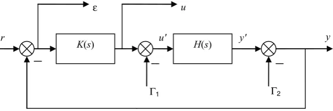
To illustrate the concept, the specification of the servo-loop’s performances can be based on the arrangement shown in Figure 1.1, which includes:

– the model’sinputdisturbances,Γ1;

– the model’soutputdisturbances,Γ2;

(24)

2 Loop-shaping Robust Control

– the value to be controlled,y, for which we have a measurement; – the measuring errorε;

– the commanducreated by the controllerK(s), whose output disturbed byΓ2is

really applied to the transfer function systemH(s).

u

Γ2

Γ1

H(s)

K(s)

r y

ε

u' y'

Figure 1.1.General view of control system

The task of an automation engineer is then to determine a controllerK(s) which, when looped withH(s), minimizes the errorεat the cost of “reasonable” commands, with the looping being subject to the external inputsr,Γ1andΓ2.

As regards the external inputs, the control and error signals are written as1_:

1 1 2 2

( ) ( ) ( ) ( )

r y y y

r

r u u u

y s H r s H s H s

s H r s H s H s

u s H εr s H ε s H ε s

Γ Γ

ε Γ Γ

Γ Γ

→ → →

= + +

Let us now detail the different transfers involved.

1.1.2.1.Output sensitivity functions

At the system’soutput, we can write:

(

)

(

)

(

)

(

)

(

)

(

)

2 1

1 1 1

1 2

( ) ( ) ( ) ( ) ( )

( ) ( ) ( ) ( )

y s s H s K r s y s

s H s HKr s HKy s

I HK y s s H s HKr s

y s I HK HKr s I HK H s I HK s

Γ Γ

− − −

= − + − + −

= − − + −

+ = − − +

= + − + − +

(25)

The Loop-shaping Approach 3

and:

(

)

(

)

(

)

(

)

(

)

(

)

(

)

(

) (

(

)

(

)

(

)

(

)

(

)

(

)

1 1 1

2 1

1 1 1

2 1

1 1 1

2 1

1 1 1

1 2

( ) ( ) ( )

( ) ( ) . ( ) ( )

( ) ( ) ( )

( ) ( ) . ( )

( ) ( ) ( )

s r s y s

r s I HK s I HK H s I HK HKr s

I I HK HK r s I HK s I HK H s

I HK I HK HK r s I HK s I HK H s

I HK r s I HK H s I HK s

ε

Γ Γ

− − −

= −

= + + + + − +

= − + + + + +

= + + − + + + +

= + + + + +

In addition:

(

)

1

(

)

1

(

)

1

1 2

( ) ( )

( ) ( ) ( )

u s K s

K I HK r s K I HK H s K I HK s

ε

Γ Γ

− − −

=

= + + + + +

Denoting the output2_{sensitivity functions as follows:}

1 1

( ) , ( )

y y

S = +I HK − T = +I HK − HK [1.1]

Thus we obtain:

1 2

( ) ( ) ( ) ( )

y y y

y s T r s S H s S s

s S r s S H s S s

u s KS r s KS H s KS s

Γ Γ

ε Γ Γ

Γ Γ

= − −

= + +

As there is no reason for the productKHto be equal toHKin the MIMO case, we can obtain other expressions for the above signals.

1.1.2.2.Input sensitivity functions

At the system’sinput, we can write:

(

)

(

)

(

)

(

)

(

)

(

)

2 1

1 1 1

1 2

( ) ( ) ( ) ( ) ( )

( ) ( ) ( ) ( )

( ) ( ) ( )

u s K r s s H s u s

Kr s K s KH s KHu s

I KH Kr s I KH KH s I KH K s

Γ Γ

− − −

= − − + − +

= + + −

(26)

4 Loop-shaping Robust Control and:

(

)

(

)

(

)

(

)

(

)

(

)

(

)

(

)

(

)

(

)

(

)

(

)

(

)

1

1 1 1

2 1 1

1 1 1

2 1

1 1 1

2 1

1 1 1

1 2 '( ) ( ) ( ) ( ) ( ) ( ) ( ) ( ) ( ) ( ) ( ) ( ) ( ) ( ) ( ) ( )

u s u s s

I KH Kr s I KH K s I KH KH s s

I KH Kr s I KH K s I KH KH I s

I KH Kr s I KH K s I KH KH I KH s

I KH Kr s I KH s I KH K s

Γ Γ Γ Γ Γ Γ Γ Γ Γ Γ − − − − − − − − − − − − = − = + + + + + − = + + + + + − = + + + + + − + = + − + + + Furthermore:

(

)

(

)

(

)

(

)

(

)

(

)

2

1 1 1

1 2 2

1 1 1

1 2

( ) '( ) ( )

( ) ( ) ( ) ( )

( ) ( ) ( )

y s Hu s s

H I KH Kr s H I KH s H I KH K s s

H I KH Kr s H I KH s H I KH K I s

Γ Γ Γ Γ Γ Γ − − − − − − = − = + − + + + − = + − + + + − Finally:

(

)

(

)

(

)

(

)

(

)

(

)

(

)

1 1 1

1 2

1 1 1

1 2

( ) ( ) ( )

( ) ( ) ( ) ( )

( ) ( ) ( )

s r s y s

r s H I KH Kr s H I KH s H I KH K I s

I H I KH K r s H I KH s H I KH K I s

ε Γ Γ Γ Γ − − − − − − = − = − + + + − + − = − + + + − + −

By setting the following as input sensitivity functions3_:

(

)

1

( ) ,

u u

S = +I KH − T = +I KH − KH [1.2]

then:

(

)

(

)

1 1

(

2

)

2

1 2

( ) ( ) ( ) ( )

u u u

y s HS Kr s HS s HS K I s

s I HS K r s HS s HS K I s

u s S Kr s T s S K s

Γ Γ ε Γ Γ Γ Γ = − + − = − + − − = + +

Hence, finally, we obtain:

1 2

r y y u y y u y y u

r y u y u y u

r u y u u y u u y u

H T HS K H S H HS H S HS K I

H S I HS K H S H HS H S I HS K

H KS S K H KS H T H KS S K

ε ε ε → → → → → → → → → = = = − = − = − = − = = − = = = = − = = = = = =

(27)

From this, we can draw the following fundamental relations:

y u u y

y y u u

T HS K T KS H

S H HS S K KS

S T I S T I



= = 

 _



=  = 

 

+ = _ + = _

[1.3]

It should be noted that in the case of positive output feedback, we repeat all the previous steps, replacingrwith -randKwith -K, from which we draw the following relations:

y u u y

y y u u

T HS K T KS H

S H HS S K KS

S T I S T I



= − = − 

 



=  = 

 

+ = _ + = 

where:

(

)

1

1 1

( ) ,

( ) , ( )

u u

y y

S I KH T I KH KH

S I HK T I HK HK

− −

= − = − −

1.1.3.Declination of performance objectives

In view of the previous developments, by frequency modeling only the direct (S) and complementary (T) sensitivity functions, we are therefore able to model all the closed-loop transfers, because they depend only on these functions. Thus, the work on many transfers can be assimilated to work on the two sensitivity functionsSand

T.

In addition:

– when σ

(

HK

)

>>1 or when σ

(

KH

)

>>1 (which can happen, particularly in low frequencies in the presence of integrators in the control law), then:

( )

(

)

(

)

( )

(

)

(

)

1

1 _,

y y

u u

S H K T I

H K

S K H T I

K H

σ σ

σ

σ σ _σ

−

≈ = ≈

(28)

and4_:

( )

(

)

( )

(

)

( )

( ) 1 ( ) ( ). ( ) . ( ) 1 ( ) ( ). ( ) y y u u H S H HK K K KS

HK H K H

H H S

KH

K K

S K

KH K H H

σ σ σ σ σ σ σ σ σ σ σ σ σ σ σ σ σ σ σ σ ≈ ≈ ≤ ≈ ≈ ≈ ≤ ≈

Then, in relation to the open-loop response in the model’s output, we obtain:

(

)

(

)

(

)

(

)

(

)

(

)

( )

(

)

(

)

(

)

1 2 1 1 2 2 1 1 ( ) ( ) 1 ( )

r y u

r u u

y y r H H H H H H H H HK

H H H

HK ε ε ε σ σ σ σ σ σ σ σ _σ σ σ σ σ → → → → → → → → → = ≈ = ≈ = ≈ = = ≈

but also for the input ones:

(

)

(

)

(

)

(

)

(

)

(

)

( )

(

)

(

)

(

)

1 2 1 1 2 2 1 1 ( ) ( ) 1 ( )

r y u

r u u

y y r H H H H H H H H KH

H H H

HK ε ε ε σ σ σ σ _σ σ σ σ σ σ σ σ σ → → → → → → → → → = ≈ = ≈ = ≈ = ≈ ≈

4 Remember that:

( ) ( )

( )

( ) ( )

( )

1 1 1 1 1

if A exists, 1

B C BC BC B C

A A

A

A A A

(29)

Thus, by giving the open loop a high gain through its singular values, the automation engineer can favor the performance of looping in relation to the external inputs by way of all the transfers relating to the errorε(H₁_→_ε,H₂_→_ε and H_r_→_ε) but has no flexibility on transfers relating to the control signal which do not depend on the open-loop response.

– when σ

(

HK

)

<<1 or when σ

(

KH

)

<<1, (which can happen, particularly in high frequencies in the presence of roll-off filters in the control law), then:

( )

(

)

( )

(

)

, , y y u u

T HK S I

T KH S I

σ σ σ σ ≈ ≈ ≈ ≈ and:

( )

(

)

(

)

( )

(

)

( )

(

)

(

)

( )

( ) ( ) y y u u HK KS K H

S H H

KH

S K K

H HS H σ σ σ σ σ σ σ σ σ _σ σ σ ≈ ≈ ≈ ≈ ≈ ≈

Then, in relation to the open loop at the model’s output, we obtain:

(

)

(

)

(

)

(

)

(

)

(

)

(

)

(

)

( )

(

)

(

)

(

)

1 2 1 1 2 2 ( ) 1

r y u

r u u

y

r y

H H HK

HK

H H

H

H H H

ε ε ε σ σ σ σ σ σ σ σ σ σ σ σ σ → → → → → → → → → = ≈ = ≈ = ≈ = = ≈

but also at the input:

(

)

(

)

(

)

(

)

(

)

(

)

(

)

( )

(

)

(

)

(

)

1 2 1 1 2 2 ( ) ( ) 1

r y u

r u u

y

r y

H H KH

KH

H H

H

H H H

(30)

Thus, by giving the open loop a low gain through its singular values, the automation engineer can favor the command of the looping (in terms of power consumption) in relation to the external inputs by way of all the transfers relating to the control signalu (H₁_→_u,H₂_→_u and H_{r u}_→ ) but has no flexibility on transfers relating to the error which do not depend on the open-loop response.

Thus, the “loop-shaping” approach consists of appropriate modeling of the singular values of the open loop response so as to guarantee certain specifications relating to Su,yand Tu,y, which themselves are derived from the declination of the set of specifications relating to all the loop transfers. Indeed, it is simpler to model a single transfer function (the open loop) than a multitude of closed-loop transfers.

The approach is particularly advantageous for the robustness of any looping that is subject to external inputs. Indeed:

– desensitizing the error ε to disturbances consists of giving Su,y a rejection

behavior on the frequency dynamics of these disturbances, i.e. giving the singular values of the open loop a high gain within the same frequency range;

– desensitizing the control signal u to disturbances consists of giving Tu,y a

rejection behavior on the frequency dynamics of these disturbances, i.e. giving the singular values of the open loop a low gain within the same frequency range.

Disturbance rejection problems can therefore, theoretically, be easily solved by including low-pass and high-pass filters in the shape of the open-loop response, depending on which axis of synthesis is favored (control signal or performance), which renders this approach particularly attractive in the world of industry.

1.1.4.Declination of the robustness objectives

It is necessary to combine the concept of robustness with the above declination of performance objectives when the looped system is subject to uncertainties (neglected time-constants, parametric variations, etc.).

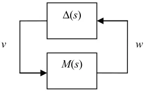
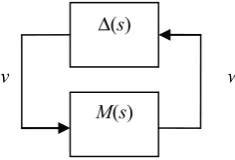
Consider the standard arrangement as shown in Figure 1.2. Analysis of the stability robustness of the system M(s), subject to unstructured uncertainties Δ(s), can be performed with the help of the small-gain theorem [ZHO 96]. Considering that M s( )∈RH_∞ and Δ( )s ∈RH_∞, the system is stable for any Δ(s) such that

1

( )s

Δ _∞ ≤γ− iff: ( )

(31)

The uncertainty block Δ(s) is therefore seen as being an internal disturbance which could destabilize the system, whereas in the previous section the signalsr,Γ1

and Γ2 were external disturbances. A similar declination methodology can be

established to complement the previous one.

Δ

(

s

)

M

(

s

)

w

v

Figure 1.2.Standard form for robustness analysis

Six types of representation of unstructured uncertainties are usually employed: – Direct multiplicative uncertainty:

- at input (Figure 1.3):

H

(

s

)

K

(

s

)

Δ

i

(

s

)

w

v

Figure 1.3.Direct multiplicative uncertainty at input

In this case, we achieve a representation similar to Figure 1.2 by using the relations:

u y

(32)

- at output (Figure 1.4):

H(s)

K(s)

Δo(s)

w v

Figure 1.4.Direct multiplicative uncertainty at output

In this case:

y u

w T v HS Kv= =

According to the small-gain theorem, with this type of representation of uncertainties, the looped system is internally stable if:

( )

0 1

1 y

u

i

T

σ

σ Δ σ

σ Δ <

<

When σ

( )

HK <<1 or when σ

(

KH

)

<<1 (which can happen, particularly in high frequencies in the presence of roll-off filters in the control law), then:

( )

(

)

, ,

y y

u u

T HK S I

T KH S I

σ σ

≈ ≈

In this case, the condition of stability robustness in relation to uncertainties represented in direct multiplicative form can be taken into account in the loop-shaping specification as follows:

( )

(

)

( )

0

1

1 i

HK

KH

σ

σ Δ σ

σ Δ

(33)

This enables us to position the roll-off necessary for the open loop to ensure the condition of stability robustness.

– Inverse multiplicative uncertainty: - at input (Figure 1.5):

H(s)

K(s)

Δi(s)

w v

Figure 1.5.Inverse multiplicative uncertainty at input

In this case:

u

w S v= ;

- at output (Figure 1.6):

H(s)

K(s)

Δo(s)

w v

Figure 1.6.Inverse multiplicative uncertainty at output

In this case:

y

(34)

According to the small-gain theorem, with this type of representation of uncertainties, the looped system is internally stable if:

( )

0

1

1 y

u

i

S

σ

σ Δ σ

σ Δ

< <

When σ

(

HK

)

>>1 or when σ

(

KH

)

>>1 (which can happen, particularly at low frequencies in the presence of integrators in the control law), then:

( )

(

)

(

)

( )

(

)

(

)

1

1 _,

y y

u u

S H K T I

H K

S K H T I

K H

σ σ

σ

σ σ

σ

−

≈ = ≈

In this case, the condition of stability robustness in relation to uncertainties represented in inverse multiplicative form can be taken into account in the loop-shaping specification as follows:

(

)

( )

(

)

( )

(

)

( )

(

)

( )

0 0

1 1

i i

H K H K

K H K H

σ σ Δ

< ⇔ >

−Direct additive uncertainty (Figure 1.7):

H(s)

K(s)

Δ(s)

w v

(35)

In this case:

u y

w S Kv KS v= =

Whenσ

(

HK

)

<<1 or whenσ

(

KH

)

<<1, then:

(

)

(

)

(

)

(

)

, ( )

y y

u u

H K

K S S I

H K H

S K S I

H

σ σ

σ _σ

≈ ≈

In this case, the condition of stability robustness in relation to uncertainties represented in direct additive form can be taken into account in the loop-shaping specification as follows:

(

)

( )

(

)

( )

( ) i

H H K

H K H

σ σ

σ Δ σ σ

σ Δ

< <

−Inverse additive uncertainty (Figure 1.8):

H(s)

K(s)

Δ(s)

w v

Figure 1.8.Inverse additive uncertainty

In this case:

y u

(36)

When σ

( )

HK >>1 or when σ

(

KH

)

>>1 (which can happen, particularly at low frequencies in the presence of integrators in the control law), then:

(

)

( )

(

)

( )

,

( )

,

( )

y y

u u

H

S H T I

H K H

H S T I

K H

σ σ

σ σ σ

σ

≈ =

In this case, the condition of stability robustness in relation to uncertainties represented in inverse additive form can be taken into account in the loop-shaping specification as follows:

( )

(

)

( )

(

)

( )

1

( )

1

( )

H

H K

H K H

H

K H

K H H

σ _σ σ Δ

σ σ Δ σ

σ σ Δ

σ

σ σ Δ σ

< ⇔ >

Thus, we have demonstrated how unstructured uncertainties can be taken into account in the loop-shaping approach, which is a welcome addition to the declination of performances presented above, with the simplicity of the approach also being an asset: modeling a single transfer (the open-loop response) enables us to implement loops that perform in relation to external signals as well as that are robust in relation to uncertainties.

1.2. Generalized phase and gain margins

Continuing with the open-loop response modeling approach, we can seek to extend the concepts of gain and phase margins to the case of multivariable systems.

1.2.1.Phase and gain margins at the model’s output

H(s)

K(s)

r _Λ y

s

(37)

What are the maximum acceptable variations in gain and phase at the model’s output which would destabilize the loop shown in Figure 1.9, in which we consider:

(

)

diag j i, 1,..,

s k ei φ i p

Λ = =

Nominally: 0 0 i

s i

k

I

Λ φ

= 

 =

 = _

We can represent this uncertainty in direct multiplicative form at output (Figure 1.4).

Thus, we have:

(

)

diag 1 j i, 1,..,

s I o o I s k ei φ i p

Λ = −Δ Δ = −Λ = − =

We set:

1 1

( )

y

T s α

∞

=

Hence, according to the small-gain theorem, the system is stable if:

1 1 j i 1

o k ei φ

Δ _∞<α ⇔ − <α Whenφ =_i 0, this condition leads to:

1 1

1−α < < +k_i 1 α

Similarly, when k_i =1:

2 2

1 1 1

1 2 sin

2

i i

i j j

j i

e e e

φ φ

φ _α − _α  φ _α

− < ⇔ − < ⇔ _{ } <

 

so:

1 2arcsin

2

i α

(38)

In addition, the uncertainty can be represented in inverse multiplicative form at output (Figure 1.6).

Thus, we have:

(

)

1 1 1

0 diag 1 j i 1, 1,..,

s o s s

i

I I I e i p

k φ

Λ ₌ ₊Δ − _⇔Λ− _{= +}Δ _{⇔ =}Δ Λ− _{− =} _ − ₋ ₌ _

 

We set:

2 1

( ) y

S s

α

∞

=

Hence, according to the small-gain theorem, the system is stable if:

0 2 1 j i 1 2

ie

k φ

Δ _∞ <α ⇔ − − <α

Whenφ_i =0, we obtain 1 1 ₂ i

k − <α , which leads to:

2 2

1 1

1+α <ki <1−α

When k_i =1, ₁ ₂ 2 2 ₂ _{2 sin} ₂

2

i i

i j j

j i

e e e

φ φ

φ _α − _α φ _α

− _{− <} _ ₋ _< _   _<

 

  ; thus:

2 2arcsin

2

i α

φ <  

 

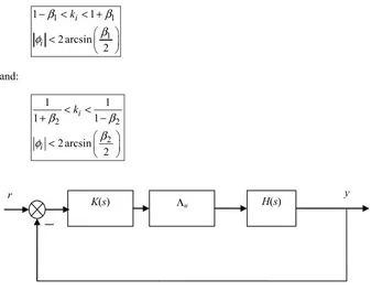
1.2.2.Phase and gain margins at the model’s input:

We now look for the maximum acceptable variations in gain and phase at the model’s input which would destabilize the loop shown in Figure 1.10, in which we consider:

(

)

diag j i, 1,.., u k ei φ i m

(39)

By setting:

1

2 1 ( )

1 ( ) u

u

T s

S s

β

∞

= =

A process strictly similar to the one outlined above establishes the following conditions:

1 1

1

1 1

2arcsin 2 i

i

k

β β

β φ

− < < +

 

< _ _

 

and:

2 2

2

1 1

2arcsin 2 i

i

k

β β

β φ

< <

+ −

 

< _ _

 

Λu K(s)

r _H₍_s₎ y

Figure 1.10.Generalized phase and gain margins at the model’s input

1.3. Limitations inherent to bandwidth

We shall now speak of a limitation inherent to the bandwidth attainable when the system in question has a certain number of unstable polespiand/or a certain number

of unstable zeroszi. [SKO 01] shows that the attainable bandwidthωBPmust be such

(40)

( )

Re( ) 0 Re( ) 0

ma ω max

i i

i BP i

p z

x p z

> >

< < [1.4]

1.4. Examples

Below, we give a few examples of typical variants of the loop-shaping technique. For simplicity’s sake, we shall work with a monovariable system. This being the case, it is clear that:

u y

S S S

T T T

= =

1.4.1.Example 1: sinusoidal disturbance rejection

Suppose we wish to set the valueyat 0 and we assume that the loop is subject to a disturbance at the model’s output Γ2( )s represented as a sinusoidal signal of amplitude Γ₀ and frequency ω₀ (e.g. local mechanical deformation, etc.). The aim is to determine a loop-shaping specification for the servo-loop; therefore, we shall focus successively on two areas: performance and then command.

Two axes for synthesis may be envisaged, depending on the “high-level constraints”:

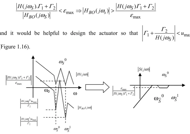
– first case: it is of crucial importance, when good performance is required, to desensitize the error ε, which must remain below a certain value ε_max.

If we set the following for the open-loop response: H_BO( )s =H s K s( ) ( ), then

2 ( ) ( ) ₁ 1 _{( )} BO

H s S s

H s

ε

→ = = ₊ must exhibit rejection behavior in ω0, which is possible if the open loop is high-gain at this frequency, because in this case:

0

0 1

( )

BO

S j

H j

ω

≈ . The specification on the error thus imposes the gain of the open loop in ω₀, because:

0 0

0 max 0

0 max

( ) ( )

( ) BO

BO

S j H j

H j

Γ Γ

ω ε ω

ω ε

(41)

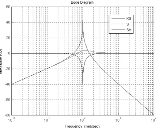
This enables us to determine the level of gain needed for the open-loop response to lendSthe desired depth of rejection in ω₀ (see Figure 1.11).

ω ω0

( )

BO

H jω

0 max

Γ ε

( )

S jω

ω ω0

max 0

ε Γ

Figure 1.11.Loop-shape for sinusoidal disturbance rejection on performance

Note that the actuator therefore needs to be chosen such that it can respond to a command equal to:

max ( 0) max

u = K j

ω ε

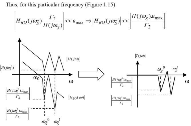
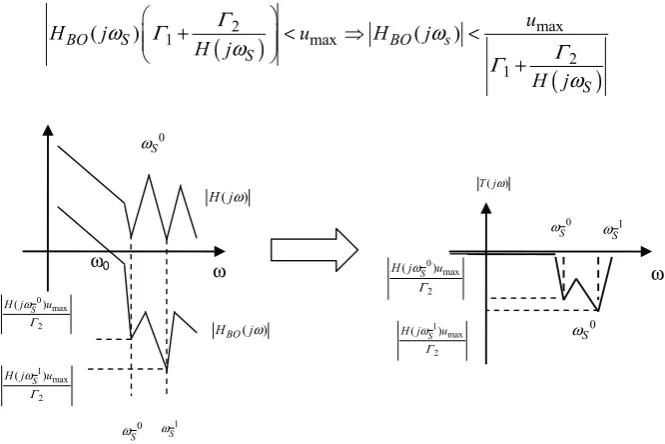
– second case: it is crucial to protect the integrity of the system and therefore to desensitize the command signalu, which must never surpass a given value umax.

Thus, 2

( ) _{( ) ( )} ( )

( ) 1 BO( )

u s _{K s S s} K s

s H s

Γ = = + must exhibit rejection behavior in

ω

0,

which is possible if the open loop is low-gain, because in this case:

0 0

0 0 0

0 0

( ) ( )

( ) ( ) ( )

( ) ( )

BO

H j T j

K j S j K j

H j H j

ω ω

ω ω ω

ω ω

≈ = ≈ . Again, the specification on the control signal imposes the gain of the open loop in ω₀ because:

0 0

0 max 0 max

0 0

( )

( ) ₍ ₎

( )

BO

BO H j

H j _u _H _j _u

H j

ω ω

Γ ω

ω <  < Γ

(42)

ω

( )

T jω

ω ω0

0 max

0

( )

H j

u ω

Γ

ω0

( ) BO

H jω

0 max

0

( )

H

Loop shaping Robust Control Free ebook download

Loop-shaping

UK USA

Table of Contents

APPENDICES. . . 245

Introduction

I.1 Presentation of the book

I.2. Notations and definitions

Chapter 1

1.1. Principle of the method

1.1.3.Declination of performance objectives

1.1.4.Declination of the robustness objectives

1.2. Generalized phase and gain margins

1.2.2.Phase and gain margins at the model’s input:

1.3. Limitations inherent to bandwidth

1.4.1.Example 1: sinusoidal disturbance rejection