NUMERICAL MODELLING OF THE ISOLATED
CURRENT LEADS FOR CRYOGENIC APPLICATIONS
by Ioan Popa, Florian Ştefănescu
Abstract. The article presents the mathematical models and the results obtained has the numerical modelling of the thermal status of the electrical leads isolated for cryogenic applications. Model them mathematics are based on the equation of thermal conduction 1D and 2D. For the numerical resolution of the thermal conduction equation one uses the finite volumes method. The elaborate program permits to get the distribution of the temperature and the flux heat along the lead as well as the low by thermal conduction to the extremities of the current way. The results obtained is using for the optimization of these current leads.
Keywords: Numerical modelling, finite volumes method, current leads, cryogenic applications.
1. Introduction
To the applications cryogenic electrotechnics of high power (cryotron, transformer, cable). they are necessary of the current ways for very high intensities. The leads them that transport high currents to the outside temperature (about 300 K) from the temperature of the cryogenic enclosure (77 K) create losses of heat that must be minimized. These losses are caused same the time by the thermal conduction due the difference of temperature between the extremities and by the effect Joule due the passage of the current. Is possible to minimize the effect Joule increasing the cross section of the electric leads, but it increase of the losses by thermal conduction. The optimal solution is obtained a balance between these two effects.
The efficient possibility to reduce the losses are cooling the leads by the cold gas that escapes of the cryogenic liquid bath (helium, hydrogen, nitrogen) [1]. In this article we considers that the lead is cooled by the liquid nitrogen that has the same temperature in all of the cryogenic enclosure (77 K).
The choice of the cooling liquid takes into account the insurance of the electric insulation.
achieved analysis one used two types of mathematical models, a simplified model (1D) and a model 2D.
2. Mathematical models
2.1. 1D Model
We considered a cylindrical lead (in copper), by the cross section A and the length, L charged by the intensity I in a cryogenic enclosure (Fig. 1). On the whole lead length is an exchange of heat by convection, characterized by the coefficient hΣ.
The distribution of the temperature on the lead’s length is governed by the equation:
(
)
( ) 0)
( − − + ρ 2 =
λ Σ T T∞ T J
A p h dx dT T dx
d
(1)
where λ - the thermal conductivity, ρ - the electric resistivity, p - the lead's perimeter, T∞ - the temperature of the cooling fluid (77K), J - the density of the current.
The electric electric resistivity has been calculated, supposing a linear variation with the temperature, by the following relation:
(
1 ( 293))
)
( = ρ293 + α −
ρT R T
The thermal conductivity can be calculated using the relation of Wiedemann-Franz:
) ( ) (
T LT T
ρ = λ
where L = 2.45⋅10−8 V2 /K2 is Lorenz's constant.
Fig. 1. Lead in a cryogenic enclosure
Fig. 2. Exchange coefficient by convection versus the difference of
temperature
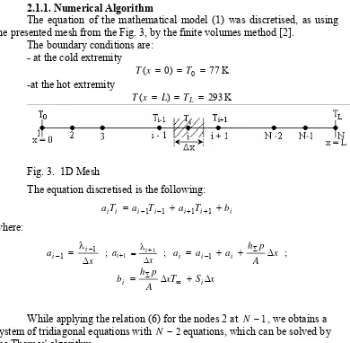
2.1.1. Numerical Algorithm
The equation of the mathematical model (1) was discretised, as using the presented mesh from the Fig. 3, by the finite volumes method [2].
The boundary conditions are: - at the cold extremity
K -at the hot extremity
K
The equation discretised is the following:
i system of tridiagonal equations with N − 2equations, which can be solved by the Thomas' algorithm.
2.1.2. Results
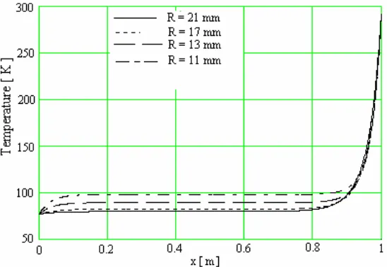
On the basis of the algorithm describes above, a program in Fortran has been elaborated. For different radius of the lead and a current I =10kAwe obtains the distribution of the temperature presented in the Fig. 4.
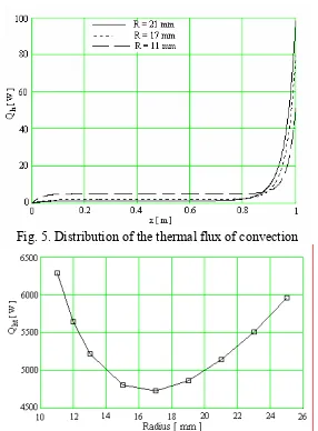
In the Fig. 5 it presents, for different radius of the lead, the distribution of the thermal flux of convection Qh of the current crossing toward the
In the Fig. 6 it presents the variation of the total convection flux Qht, between the current lead and the cryogenic liquid, versus the lead's radius.
2.1.3. Conclusion
The optimization of a cryogenic lead for a current I it makes by the good choice of the material of the lead and the cryogenic fluid, and its dimensioning. The Fig. 6 shows that there is an optimum radius for which the losses by convection are minimal. The flux of conduction at the cold extremity
0
Q , for the values of the radius between 11 mm and 25 mm, vary between 0.0177 W/A and 0.00479 W/A.
Fig. 5. Distribution of the thermal flux of convection
Fig. 6. Total flux of convection versus the lead's radius 2.2. 2D Model
We considers the thermal conduction equation 2D in cylindrical coordinates:
0 ) ( )
( )
( 1
= +
∂ ∂ ∂∂
+
∂ ∂
∂∂ z S T
T T z r T r T r
r λ λ
whereS(T) =ρ(T)J2, ρis the electric resistivity of the material and J the density
of the current.
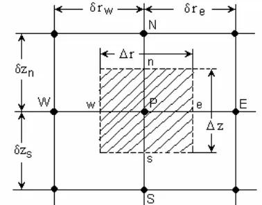
The insulation has been taken in account by an equivalent coefficient of thermal exchange by convection. As benefiting of the cylindrical symmetry of the lead, the numeric analysis domain and the mesh used is presented in the Fig. 8.
2.2.1. Numerical Method and Discretization
We uses the finites volumes method [2] for the discretization of the equation (7). To get the general form of the discretised equation, for an interior vertex of the calculation domain (the vertex 10 for example), we integrates the equation (7) on the control volume presented in the Fig. 9.
Fig. 7. Isolated cylindrical lead and the boundary conditions
∫
∫
+∫
=
∂ ∂ λ ∂∂ +
∂ ∂ λ
VC VC VC
SdV dV
z T z dV
r T r
r 0
1
∫ ∫
∫
∫
+∫ ∫
=
∂ ∂ λ ∂∂ +
∂ ∂ λ ∂∂
e
w n
s
n
s
e
w n
s e
w
dz dr Sr dz
rdr z T z dz
dr r T r
r 0 (9)
Fig. 8. Domain of calculation and the 2D mesh
The integration (9) yields:
While replacing the gradients of temperature in the equation (11), gives:
While regrouping the terms in the equation (12) we gets the general form of the discretised equation:
We obtain, of the same way, the discretised equations for the vertex situated on the West and East boundary of the calculation domain, while taking into account the boundary conditions.
The resolution of the of algebraic system of equations obtained has been achieved by using the Thomas algorithm adapted to the problems 2D [2]. The elaborated program permits the optimization of the construction of the
cryogenic current leads. 2.2.2. Results
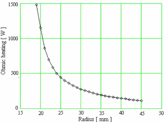
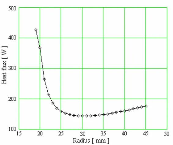
The numeric results put in evidence the lead's optimal radius. From a radius of 25 - 30 mm, the total losses by effect Joule decrease less with the lead's radius (Fig.10). One notes that the thermal flux toward the cryogenic surrounding wall (Fig. 11) has a minimal value for the radius of the lead of 30 mm. The thermal flux by the outside insulation increases very quickly (about)
W/mm
42 until the R = 23− 24mm. After this value of the radius, the thermal flux increases linear with about 10 W/mm.
Fig. 11. The thermal flux on the surface in contact with the cryogenic enclosure
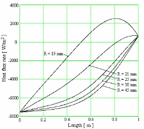
In the Fig. 13, the negative value of the heat flux means a flux coming from the outside toward the lead's inside. We also notes that from a radius of 25 - 30 mm the distribution of the density of the heat flux rate on the lead's length doesn't change practically more.
Fig. 13. The distribution of the heat flux rate by the external insulation, on the lead's length for different radius
2.2.3. Conclusions
The numerical modelling and simulation offers the possibility of the optimization of the current leads for cryogenic applications. The two models 1D and 2D show the existence of an optimal value of the lead's radius. The model 1D rather gives a qualitative description while the model 2D gives a complete description of the thermal field and therefore the possibility to calculate all thermal fluxes that participate in the thermal balance. Besides, the knowledge of the thermal flux toward the cryogenic enclosure permits the control of the use of the cryogenic liquid.
References :
[1] Donadieu L., Dammann C. (1968). Étude des traversées de courant pour enceinte cryogénique, Revue générale de l’électricité, Tome 77, No 2, Février 1968.
[2] Popa I. (2002). Modélisation numérique du transfert thermique. Méthode des volumes finis, Maison d’édition Universitaria, Craiova.
[3] Arkaharov A., Marfenina I., Mikulin V. (1981). Theory and Design of Cryogenic Systems, Mir Publishers Moscow.
[4] Popa, I., Stefănescu, F. (2003). Modélisation du régime thermique des traversées de courant cryogéniques, 4th International Conference on Electromechanical and Power Sistems, SIELMEN 2003, Chişinău, 26-27 september 2003 (Republic Moldova), pp. 155-158.
[5] Giese R.F., Runde, M. (1993). Assessment Study of Superconducting Fault-Current Limiters Operating at 77 K, IEEE Transaction on Power Delivery, Vol. 8, No. 3, July 1993, pp. 1138-1147.
[6] Hilal, M.A. (1977). Optimization of Current Leads for Superconducting Systems, IEEE Transaction on Magnetics, Vol. MAG13, No. 1, January 1977, pp. 690-693.
Authors:
Ioan Popa - University of Craiova, Romania