www.elsevier.comrlocateratmos
Stochastic effects of cloud droplet hydrodynamic
interaction in a turbulent flow
M. Pinsky
a,), A. Khain
a, M. Shapiro
b aThe Institute of Earth Sciences, The Hebrew UniÕersity of Jerusalem, GiÕat Ram, Jerusalem, Israel b
Faculty of Mechanical Engineering, Technion-Israel Institute of Technology, Haifa 32000, Israel
Abstract
The collision efficiencies of small cloud droplets are calculated in a turbulent flow. A flow
w
velocity field was generated using a model of isotropic turbulence Pinsky, M.B., Khain, A.P., 1995. A model of homogeneous isotropic turbulence flow and its application for simulation of cloud drop tracks. Geophys. Astrophys. Fluid Dyn. 81, 33–55; Pinsky, M.B., Khain, A.P., 1996.
x
Simulations of drops’ fall in a homogeneous isotropic turbulence flow. Atmos. Res. 40, 223–259 . The results indicate that in a turbulent flow the collision efficiency is a random value with high
Ž .
dispersion. The collision efficiencies depend on the initial at the infinity interparticle velocities and angles of droplet approach. The mean values of the collision efficiency and the mean values of the collision kernel in a turbulent flow exceed the values measured or calculated for still air conditions. For instance, under turbulent intensity typical of early cumulus clouds, the mean values of the collision efficiency for a 10mm drop-collector are 5 to 9 times as large as the values in the pure gravity case. In case of a 20-mm-radius drop-collector the mean collision efficiencies are greater than the corresponding gravity values by a factor ranging from 1.2 to about 6, depending on the size ratios of colliding droplets.
The collision efficiencies in a turbulent flow are shown to be very sensitive to relative droplet
Ž .
velocities. Even a small variation of about 10% of the interdrop relative velocity can result in values of the collision efficiencies twice as large as in the calm air.
Possible effects of the stochastic nature of the collision process on the evolution of the ‘‘mean’’ cloud structure are discussed. It is shown that drop concentration inhomogeneity accelerates the rate of droplet collisions, which are effective in the areas of the increased droplet concentration. To illustrate the effect of the mean increase of the collision efficiency on the drop size spectrum evolution, we solved the stochastic kinetic equation of collision. It was shown that
)
Corresponding author. Tel.:q972-2-6585822; fax:q972-2-5662581.
Ž .
E-mail address: [email protected] M. Pinsky .
0169-8095r00r$ - see front matterq2000 Elsevier Science B.V. All rights reserved.
Ž .
the increase of the collision efficiency of small cloud droplets controls the broadening of the initially narrow droplet size spectrum and accelerates the process of rain formation. The results indicate that the increase of the collision efficiency of small cloud droplets in a turbulent flow is, possibly, the mechanism responsible for in situ observed broadening of droplet spectra in undiluted cores of cumulus clouds.
In numerical simulations of drop collisions within a turbulent flow, a new effect was discovered, namely, in some cases the collision efficiencies in a turbulent flow appeared to be
Ž .
equal to zero no collisions . Analysis shows that in the case the ratio of droplet fall velocities is
Ž .
less than a certain critical value which depends on the ratio of particle sizes the falling particles form a tandem, in which particles fall with equal velocities.q2000 Elsevier Science B.V. All
rights reserved.
Keywords: Stochastical processes in clouds; Turbulence effects; Cloud microphysics; Droplet spectrum
formation
1. Introduction
1.1. Different approaches in the description of microphysical processes in clouds
When considering methods of description of microphysical processes in clouds, we can distinguish three main approaches: deterministic, ‘‘mixed’’ and fully stochastic.
A typical example of the deterministic approach is the utilization of the equation of
Ž .
continuous growth Pruppacher and Klett, 1997 . In this approach, the growth rate of large drop-collector is fully determined by the concentration of smaller droplets and terminal fall velocities of the drop-collector and small droplets. In case of equal concentration of small droplets, initially equal drop-collectors will remain equal all through the time period of their collision growth. Thus, the approach can hardly be used to reproduce the formation of a wide drop size spectrum. In numerical models, in which the equation of continuous growth is used to describe collisions of rain drops and cloud
Ž .
droplets ‘‘bulk microphysics’’ parameterization models the size spectra of rain drops
Žas well as of other hydrometeors are prescribed a priori, say, in the form of the.
Marshall–Palmer distribution. Thus, the approach is unfit to explain the process of size spectra formation of cloud hydrometeors.
An example of the ‘‘mixed’’ approach is the utilization of the stochastic kinetic
Ž .
equation of collision Pruppacher and Klett, 1997 in the so-called spectral-microphysics
Ž .
models e.g., Kogan, 1991; Khain and Sednev, 1996; Reisin et al., 1996 . In these models size distribution functions of hydrometeors of different type are calculated during the model integration. These models claim to reproduce the process of the formation of drop size spectra as well as the spectra of ice particles. The utilization of the stochastic kinetic equation of collisions means that this approach takes into account some elements of ‘‘stochasticality’’ of collision processes. The equation permits one to obtain comparably complicated shapes of size distribution of cloud hydrometeors.
Žand time resolution, drop as well as ice particles concentrations as well as the. Ž .
collision kernels used in the stochastic kinetic equation actually denote values obtained by averaging over large volumes of the order of 107 to 1010 m3. A question arises, whether microphysical processes in clouds can be described adequately under the assumption that the concentration of cloud hydrometeors and the collision kernels are constant within such large volumes.
In other words, the question is: what is the contribution of small-scale stochastic fluctuations of drop concentration and other parameters to cloud microphysics? The essence of the problem is somehow similar to the role of ‘‘subgrid’’ processes in large-scale global atmospheric circulation models. It is generally recognized that subgrid
Ž .
processes e.g., convective heating are of crucial importance when large-scale processes are simulated. The role of stochastic ‘‘subgrid’’ processes in cloud evolution is not widely recognized yet because of many uncertainties.
The third approach can be referred to as a fully stochastic one. According to this approach, drop collisions are simulated within realistic stochastic fields of velocity, concentration, supersaturation, etc., without any parameterization. The main purpose of
Ž
this approach is to understand the effects of stochastic processes on drop growth say, by
.
collisions and to find ways permitting parameterization of these fine effects in case their contribution is significant.
Ž .
Numerous recent theoretical and laboratory studies see below indicate that the impact of the small-scale stochastic effects is quite important so far as it provides an insight into some fundamental problems of cloud physics.
1.2. Turbulence effects induced by droplet inertia
The main source of ‘‘stochasticality’’ of cloud microphysical processes is cloud turbulence. Clouds are known to be areas of enhanced turbulence. Different aspects of influence of cloud turbulence on cloud evolution have been discussed in a special issue of the Atmospheric Research, Vol. 43, 1996.
We will analyze here some stochastic effects induced by the inertia of drops and ice particles moving within a turbulent flow. The problem has attracted the attention of investigators for a long time. About 50 years many studies claiming to reveal turbulence effects were criticized by other authors, therefore, no consensus has been reached toward
Ž .
1993, which has been stated by Beard and Ochs 1993 in their review. Details of the
Ž .
discussion can be found in Pinsky and Khain 1996, 1997c , Pruppacher and Klett
Ž1997 . A new splash of interest to the effects of turbulence on cloud microphysics takes.
place during a few past years.
We will mention three main mechanisms, by means of which turbulence can
Ž . Ž .
potentially influence droplet collisions: a change in the swept volume, b formation of
Ž .
concentration inhomogeneity of cloud hydrometeors and c change of the drop–drop, drop–ice and ice–ice collision efficiencies. All these turbulence effects are related to the
Ž .
drop or ice particles inertia, due to which their motion and interaction in a turbulent medium is much more complicated than in calm air.
1.2.1. Increase in the sweptÕolume
Ž .
Khain and Pinsky 1995 showed that due to their inertia drops deviate from the surrounding air parcel tracks, that is, drops in a turbulent flow never fall with their terminal fall velocities. Drops of different inertia respond differently to the wind shears of the air flow. As a result, additional drop–drop relative velocities arise leading to the
Ž .
increase of the swept volume and frequency of drop collisions. Khain and Pinsky 1995 showed that, in case of a simple background flow with the wind shear, the increase of the swept volume induced by turbulencerinertia accelerates significantly the broadening
Ž .
of the drop size spectrum by collisions. Khain and Pinsky 1997 , Pinsky and Khain
Ž1997a generalized the study to the case of a 3-D turbulent flow. Turbulence was.
assumed to be isotropic. It was shown that relative velocities between small cloud droplets were caused mainly by flow accelerations, while larger drop responded rather to flow shears. In these studies, the effects of the swept volume increase on the drop size spectrum evolution were taken into account by the increase of mean-square drop–drop relative velocities.
The increase of relative velocities and the swept volume in a turbulent flow was
Ž
shown to be especially pronounced in case of drop–ice and ice–ice collisions Pinsky
.
and Khain, 1998; Pinsky et al., 1998a . This effect can be attributed to the following. The increase in the swept volume in a turbulent flow is proportional to the ratio of inertia induced relative velocities between particles to the relative velocity induced by
Ž . Ž .
gravity. Ice particles having the same or even a larger mass inertia as compared to water drops have significantly lower terminal fall velocities induced by gravity. Thus,
Ž .
the ratio: inertia induced relative velocityrgravity induced relative velocity is higher for low-density ice particles.
1.2.2. Formation of particle concentration inhomogeneity
Ž .
Pinsky and Khain 1996 investigated drop motion in a turbulent flow using a model
Ž .
of isotropic turbulence see Appendix A . Numerous examples of drop tracks for drops of different size demonstrate a significant influence of turbulence on different aspects of drop motion. The tendency of drop tracks to collect along isolated paths was demon-strated. The existence of areas of two types within a turbulent flow was revealed. Due to their inertia, drops tended to leave the areas of enhanced flow curvature. Locating initially beyond these areas, drops tended to avoid them. At the same time drops tended to concentrate in the areas of low curvature. Thus, the effect of drop collection and formation of drop concentration inhomogeneity was demonstrated in turbulent flows typical of cloud turbulence. Spatial scales of drop concentration inhomogenieties were
Ž .
found to be dependent on drop mass inertia , so that for rain drops of a few hundred of
mm, the scales are of several meters and even tens of meters. For small cloud droplets, these scales are of one to a few centimeters.
Ž . Ž .
Earlier, Maxey 1987 and Wang and Maxey 1993 demonstrated the formation of concentration inhomogeneity of inertial particles moving within turbulent flows. In the
Ž .
last study the direct numerical simulation DNS has been used for turbulent flow generation.
Ž . Ž .
Pinsky and Khain 1997b and Pinsky et al. 1999a theoretically investigated some
Ž .
drop inertia drop flux velocity tends to be divergent even in a non-divergent turbulent flow. The drop flux divergence turned out to be maximal for drops of 100-mm radii. Drops of smaller radii follow air track of non-divergent flow more closely. The sensitivity of drops of larger size to air velocity fluctuations is lower, so that gravity induced fall velocity dominates. Thus, the rate of concentration inhomogeneity was found to be greatly dependent on the drop size. Inhomogeneities of drop concentration were most pronounced for drops of 100-mm radii. However, drop flux divergence for
Ž .
small cloud droplets 10- to 15-mm radii was found intense enough to provide significant drop concentration fluctuations, which can be of 20% to 40% of the mean drop concentration. The divergence of drop flux velocity for small cloud droplets was
Ž
found to be proportional to the dissipation rate and square of droplet radii Pinsky et al.,
.
1999a . They showed that the characteristic spatial scale of these fluctuations of droplet concentration is equal to one or a few centimeters, hence, clouds have fine structure
Ž‘‘inch clouds’’ . The mechanisms of formation of concentration inhomogeneity of.
inertial particles in different turbulent flows were studied recently by Elperin et al.,
Ž1996 , Wang et al. 1998 and Zhou et al. 1998 .. Ž . Ž .
Note that the problem of the existence of small-scale concentration fluctuations in
Ž .
clouds so-called preferential concentration remains in the cloud-physics community to
Ž
be a controversial issue see a comment of Grabowski and Vaillancourt, 1999 on the
.
paper by Shaw et al., 1998 . Recently, these centimeter-scale drop concentration fluctuations have been retrieved from a series of drop-arrival times providing in situ
Ž .
measurements using the Fast FSSP Pinsky et al., 1998b . The RMS amplitude of small-concentration fluctuation in a cumulus cloud analyzed turned out to be 30% of the mean droplet concentration, which agreed well with the theoretical evaluations of Pinsky
Ž .
et al. 1999a .
The process of collisions is known to be more effective in case of inhomogeneous
Ž .
spatial distribution of particles e.g., Voloshuk and Sedunov, 1975; Kasper, 1984 . Using a simplified model of the formation of drop concentration inhomogeneity during the
Ž .
process of drop collisions, Pinsky and Khain 1997b demonstrated a significant acceleration of the process of rain drop formation by small droplet collisions. Zhou et al.
Ž1998 demonstrated a significant increase of the collision rate of inertial particles using.
a turbulence model based on the solution of the Navier–Stokes equation.
1.2.3. Collision efficiencies of particles
One of the most efficient ways owing to which turbulence can influence microphysi-cal processes in clouds is its impact on the collision efficiencies of inertial particles. Note that in all studies mentioned above the collision efficiency was taken equal to that in the pure gravity case. In several studies the problem of hydrodynamic interaction
Ž
between droplets in a turbulent flow has been considered Almeida, 1976, 1979; Grover
. Ž .
and Pruppacher, 1985; Koziol and Leighton, 1996 . Almeida 1976, 1979 , Koziol and
Ž .
Leighton 1996 calculated the track of one drop in the vicinity of another drop under the assumption that the relatiÕe drop Õelocity at separation distances greater than
Ž .
of the order or less than the Kolmogorov microscale about 1 mm . Corresponding scales of turbulence vortices lie within the viscous subrange. According to the results
Ž .
obtained by Koziol and Leighton 1996 , the influence of such low energy vortices on the relative drop motion seems to be small.
Ž . Ž .
According to Khain and Pinsky 1997 and Pinsky and Khain 1997a , turbulence-in-duced relative velocities between drops are caused by turbulent fluctuations lying within the inertial subrange of the spectrum. Thus, drops separated by a distance of several radii in a turbulent flow have relative velocities that differ from those induced by pure
Ž .
gravitation settling. This idea was used first by Grover and Pruppacher 1985 , who investigated effects of turbulence on the ability of large rain drops to collect small particles. According to the results obtained, turbulence increases the rate at which large cloud drops collect particles in the radius range of 0.5 to 2.5mm significantly. However, the authors used a simplified one-dimensional model of turbulent flow, which limits the applicability of their results.
In a 3-D turbulent flow, the directions of drop velocities do not coincide with the direction of their approach. This factor can lead to a significant change of drop tracks during mutual approach and hence, to a significant change of the collision efficiency as compared with the case of gravitational collision.
Ž .
Vohl et al. 1996, 1999 reported the results of laboratory experiments of drop-collec-tor growth in a wind tunnel indicating a pronounced increase of drop growth rate under turbulent conditions.
Ž .
In Pinsky et al. 1999b , the hydrodynamic problem of collisions of small droplets
Žwith radii less than 30mm in a turbulent flow was analyzed. It was shown that when.
dealing with the hydrodynamic problem of drop collisions, drop-air relative velocities
Ž
formed in a turbulent flow due to drop inertia should be used as initial conditions at
.
infinity for the calculation of mutual drop tracks, and not the difference in the still air terminal velocities.
The collision efficiencies of cloud droplets were calculated using the superposition method. A certain number of calculations shows that the droplet collision efficiencies in a turbulent flow are usually larger than those in calm atmosphere. It is stressed that in a turbulent flow the droplet collision efficiency is a random value with a significant dispersion.
In the present study, we report some results concerning the stochastic nature of the collision efficiency of particles in a turbulent flow. In a special section, we discuss the possible contribution of these processes to cloud microphysics.
2. Droplets hydrodynamic interaction in a turbulent flow
Ž .
This section is based on the study of Pinsky et al. 1999b .
2.1. Conditions of droplet collisions in a turbulent flow
The motion of inertial droplets in a turbulent flow depends on wind shears and flow
Ž . Ž .
the maximum of the wind shear spectrum is reached in the transition area from the inertial to the viscous subrange that corresponds to the length scale of about 2 cm. At a smaller length scale of the wind shear spectrum sharply decreases due to the viscous effect. The maximum in the spectrum of acceleration can be expected to be located near the maximum of the shear spectrum.
The location of the maximum in a spectrum is known to be closely connected with the correlation length. The fact that the maximum of the shear and acceleration spectra are attained at 1 to 2 cm means that the correlation lengths of the velocity shear and the inertial acceleration are as small as 1 to 2 cm as well. Thus, shears, as well as flow accelerations become independent at distances greater than about 2 cm. At the same time, at distances below 1-cm shears as well as the inertial accelerations are well correlated. It means that within air volumes of these linear scales shears and inertial accelerations do not experience significant variations.
While in still air drops quickly accelerate towards their terminal fall velocity, in
Ž .
spatially non-uniform flows sheared and turbulent flows drop inertia always leads to the formation of additional non-zero velocity deviations from the surrounding flow. Thus, in a turbulent flow one can see no adaptation of drop velocity to the surrounding flow. Such adaptation does not take place because the flow itself changes in surrounding of a moving drop and the drop experiences flow accelerations during each instance of its motion. Thus, in a turbulent flow drops never fall with their terminal fall velocity. The
Ž .
adaptation relaxation period can be defined in this case as a time period during which
Ž .
initial conditions e.g., initial drop velocities influence drop velocity. When this adaptation period is over, the drop velocity and its deviation from the flow velocity
Ž
depend only on the drop mass and flow parameters such as the values of the shear,
.
curvature of air parcel tracks, flow velocity, etc. . Taking into account that the duration of relaxation periods is short, especially for small drops, changes of drop velocity deviations can be regarded as transitions from one adjusted state to a subsequent state. It means that adjusted drop velocity deviations change with the characteristic time scales of the surrounding air flow.
The time correlation scale of drop-air relative velocity can be evaluated as the lifetime of those turbulent vortices, corresponding to the maximum shears and accelera-tions of the air. The lifetime for turbulent vorticest with the linear length lwithin the inertial subrange can be evaluated as tf´y1r3l2r3
. For l of about 1 cm, t is about 0.2 s.
The interdrop relative velocity induced by the difference in drop inertia is a direct consequence of the formation of drop-air relative velocities. Thus, interdrop relative velocity has typical temporal and spatial scales similar to those for the velocity of a larger drop relative to the surrounding air.
Some characteristics of relative velocity between droplets as seen from the calcula-tions of drop motion within a turbulent flow generated by the turbulent model by Pinsky
Ž .
and Khain 1995, 1996 are presented in Figs. 1 and 2.
Fig. 1. The distribution of 10- and 20-mm-radii interdrop velocity normalized by the difference in drop
Ž .
terminal velocities as seen from the model of turbulent flow, Pinsky and Khain, 1995 .
early stage of cumulus clouds. One can see a comparably wide symmetric distribution. The relative velocities between these comparably large cloud droplets can be by 20–30% largerrsmaller than the value in the pure gravity case.
The distribution of relative velocities is accompanied by the distribution of angles at
Ž .
which drops approach Fig. 2 . Zero value of the angle corresponds to pure gravity case with the drop approach in the vertical direction. One can see that in turbulent flows the angles of drop approach can be as large as 40–508even in the comparably low intensity turbulence. As it will be shown below, these factors lead to a significant dispersion of the collision efficiencies in a turbulent flow. In a turbulent flow the collision efficiency becomes to be random value with a wide distribution.
Ž . Ž .
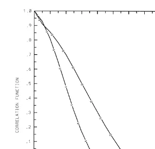
Fig. 3 shows longitudinal curve A and lateral curve B spatial correlation functions of x-component of relative velocity between 10 and 20mm -radii droplets One can see that the spatial correlation lengths are about 0.8 cm for longitudinal and 1.1 cm for lateral spatial correlation functions, respectively.
characteris-Ž
Fig. 2. The distribution of angles at which drops of 10- and 20-mm-radii approach as seen from the model of
.
turbulent flow, Pinsky and Khain, 1995 .
tic spatial and time scales of relative interdrop velocities induced by the drop inertia with the characteristic scales of hydrodynamic interaction between droplets.
Ž .
As it is known Pruppacher and Klett, 1997 , drops hydrodynamic interaction begins when drops approach at the distance of several radii of the larger drop. In this study we deal with droplets with the radii below 30 mm. Thus, the spatial scale characterizing hydrodynamic interaction between droplets is below 0.03 cm. A great number of simulations of droplets motion during their hydrodynamic interaction shows that typical
Ž
hydrodynamic interaction time the time during which droplets are separated by
dis-.
tances not exceeding several drop radii is about 0.01 s. to 0.02 s.
Thus, in case of a non-uniform flow the difference in terminal fall velocities should be added by the interdrop velocity induced by drop inertia. Besides, time and spatial correlation scales of drop-air and interdrop relative velocities in a turbulent flow are much greater than the characteristic time and spatial scale of hydrodynamic droplet interaction.
Ž . Ž .
Fig. 3. Longitudinal curve A and lateral curve B spatial correlation functions of x-component of the relative
Ž .
velocity between 10- and 20-mm-radii droplets of see, Pinsky et al., 1998c for more detail . One can see that the spatial correlation lengths are about 0.8 cm for longitudinal and 1.1 cm for lateral spatial correlation functions, respectively.
force acts similarly to the gravity force through the process of drop hydrodynamic interaction. All changes of drop velocities during hydrodynamic interaction take place only due to the mutual influence of drops.
Ž .
Thus, we will neglect the influence of turbulent vortices velocity fluctuations at scales of hydrodynamic droplet interaction. Instead, we will take into account inertia-in-duced velocities at the periphery of drop hydrodynamic interaction zone. These veloci-ties will be included into the boundary conditions when solving the hydrodynamic problem of droplet interaction.
2.2. Drop motion equations and geometry of drop collisions in a turbulent flow
The equation system and approach to the calculation of the collision efficiencies are
Ž .
To calculate the hydrodynamic interaction between two spheres moving in the air
Ž .
flow, we use here the superposition method Pruppacher and Klett, 1997 . According to this method each sphere is assumed to move in a flow field induced by its counterpart
Ž .
moving alone. Dating back to Langmuir 1948 , this method has been successfully used
Ž
by many investigators e.g., Shafrir and Gal-Chen, 1971; Lin and Lee, 1975; Schlamp et
.
al., 1976 for a wide range of droplet Reynolds numbers.
In Appendix B we show that drop motion equations describing their hydrodynamic
Ž .
interaction in a inhomogeneous for example, turbulent flows can be written in the
™
coordinate frame moving with the background velocity V as:a
™X
where indices 1,2 denote the number of droplets, V is drop-air relative velocity of ithi
Ž .
drop is1,2 ,tisVi trg is the characteristic relaxation time of ith drop. This time is a™
™ ™
measure of drop inertia. V is the velocity of ith drop, u and ui 1 2 are the perturbed velocity fields induced by drop 1 in the point of the location of the center of drop 2, and
™
by drop 2 in the point of the location of the center of drop 1, respectively, so u2rt1 is the acceleration caused by air velocity perturbations induced by the second drop.™
X
Ž .
In Eqs. 2.1–2.2 , velocity Vi` can be interpreted as a relative drop-air velocity of ith droplet at sufficiently large distances where the velocity field induced by the other drop in a drop pair can be neglected.
Ž .
The system 2.1–2.2 is similar to a corresponding one usually used for the calculations of the collision efficiency by the superposition method in the pure gravity
Ž .
case e.g., Lin and Lee, 1975 . The difference is that the drop velocity at infinity is not equal to the terminal fall velocity. For example, for drop 1:
™ ™
dV dV
™X ™ a ™ a
V1`sV1 , tezyt1 st1
ž
gy/
.Ž
2.3.
d t d t
This velocity can be interpreted as a relative drop-air velocity of droplet 1 at sufficiently large distances, where the velocity field induced by drop 2 can be neglected. V1 t is the
™
terminal velocity of drop 1 in calm atmosphere, e is the unit vector directed downward.z This condition is the boundary condition at infinity. Since the spatial correlation scale of these inertia-induced velocities is 1 to 2 cm for small droplets, these velocities may be assumed constant at the distances of drop dynamic interaction. They also can be
™
Ž .
assumed to be time-independent. The term yt1dVard t in Eq. 2.3 is actually an additional relative drop velocity induced by the drop inertia. This parameter, which was not taken into account in earlier studies, is of crucial importance since it determines the
™
™ ™
Ž .
The term gydVard t does not change during the process of drop hydrodynamic interaction and can be interpreted as ‘‘modified gravity’’. In case illustrated in Fig. 1, mean deviations of ‘‘modified gravity’’ from pure gravity are about 20 %, but in some cases they can exceed 40%.
The geometry of droplet approach corresponding to the droplet motion equations is as
X X X4
follows. We consider the droplet motion in the coordinate frame x , y , z moving with the velocity of the background flow. The frame is oriented in such a way that the z-axis should be directed anti-parallel to the relative velocity.
Ž .
Fig. 4a,b illustrates the definition of the collision efficiency in case a of a turbulent
Ž . X X X4
flow and b calm air, respectively. We consider drop motion in the frame x , y , z
™
moving with the background flow velocity V . The frame is oriented in such a way that™ a ™
X X X X
4
the x , z™plane should contain vectors V™ ™ 1` and V , and, correspondingly, the relative2`
X X X
velocity V12`sV1`yV . This approach permits one to reduce the three-dimensional2`
Ž . 1
drop interaction problem to a symmetric geometry quasi two-dimensional problem. In the turbulent case, xX-components of relative drop velocities at the infinity are
X X X4
non-zero but equal to each other, as a result of the choice of the x , y , z coordinate frame. The z™ X-axis can have any direction depending on the direction of relative velocity
V12`. It is important that droplets approach does not coincide with the directions of drop velocities at infinity. ™
In case of still air the vector V12` is the difference in the droplets terminal velocities. In a turbulent flow, the drop-air relative velocities are oriented at angles a1 and a2
Ž .
relative to their approaching direction Fig. 4a . These angles are determined by the
™X ™
directions of drop velocities with respect to the surrounding air velocities: V™ 1`yu and2
X ™ X X4
V2`yu . The x , z1 plane is a symmetry plane for the flow fields induced by moving droplets. This symmetry arises due to the fact that the velocity fields induced by the
Ž .
moving droplets are axisymmetric see Appendix B .
X X4
Droplets initially located in the plane x , z will remain within this plane during drop approach. If one of the droplets does not initially lie in this plane, its track will not lie in the plane either. In this case there exists a point symmetric to the initial position of the drop with respect to this plane. A drop put at the point will have a track symmetric to the track of the first drop with respect to the plane. In other words, droplet motion during their hydrodynamic interaction appears to have a mirror symmetry with respect to
X X4
the x , z plane.
In the pure gravity case the geometry of drop interaction is axisymmetric with respect
X Ž .
to z axis Fig. 4b . One can see that the determination of the collision cross-sections and the collision efficiencies in a turbulent flow can be defined in a manner similar to the case of pure gravity collisions. Fig. 4c,d illustrates the definition of the collision efficiency in a turbulent flow and calm air, respectively. In pure gravity case grazing
X Ž .
tracks are axisymmetric with respect to the z -axis Fig. 4d . In a turbulent flow segment
Ž X .
Xc extension of the collision cross-section in the x -direction is located asymmetrically
X Ž .
with respect to the z -axis Fig. 4c .
™X ™X
1
Ž . Ž .
Fig. 4. Illustration of the definition of the collision efficiency in case a of a turbulent flow and b calm air,
X X X4 4
respectively. The x , y , z coordinate frame moving with respect to the immovable x, y, z frame with the
™ X ™X
velocity of the background flow V and with z axis directed anti-parrallel to relative velocity Va 12`. We define™
X X X X X
4 Ž .
the x , z™ plane the x axis is perpendicular to the z axis in such a way that it contains both vectors V1`and
X X Ž .
V . While in the pure gravity case grazing tracks are axisymmetric with respect to the z axis b , one can2`
Ž X .
show that in a turbulent flow segment the extension of the collision cross-section in x -direction will be
X Ž . Ž .
located asymmetrically with respect to the z axis a see Pinsky et al, 1999b for more detail . The definition
Ž . Ž .
of the collision efficiency in c a turbulent flow and d calm air. While in the pure gravity case grazing
X Ž .
tracks are axisymmetric with respect to the z axis d , one can see that in a turbulent flow segment Xc
Ž X . X Ž .
The grazing tracks form the effective collision cross-section of area S on the planec perpendicular to the direction of interdrop relative velocity at infinity. In case of a turbulent flow the effective collision cross-sections are not circular and can be shifted
X X X4
with respect to the z -axis, remaining, however, symmetric with respect to the x , z plane.
The collision efficiency in a turbulent flow E is calculated as the ratio of S to thet c
Ž .2 geometric cross-sectionp a1qa2 :
2
EtsScrp
Ž
a1qa2.
Ž
2.4.
where a and a are the radii of interacting droplets. The collision efficiency for pure1 2 gravity collisions E is determined in a similar way, but allowing for the axisymmetricg geometry it can be calculated as:
2 2
EgsYcr4 a
Ž
1qa2.
.Ž
2.5.
In this case the collision cross-section is a circle with the center located on the zX-axis.
X X4 X X4
The linear collision efficiency in x , z and y , z planes can be defined as
ExsXcr 2 a
Ž
1qa2.
Ž
2.6a.
and
EysYcr 2 a
Ž
1qa2.
,Ž
2.6b.
respectively. As it was mentioned above, segment Y is located symmetrically relative toc
X X4 w Ž .x
the x , z plane. In calm air ExsEysYcr2 a1qa2 . In a turbulent flow Ex is usually not equal to E .y
3. Results of calculation of the collision efficiencies in a turbulent flow
In the calculations the dissipation rate of turbulent kinetic energy was taken equal to 100 cm2 sy3, typical of early cumulus clouds.
The calculation of the collision efficiency was carried out in two steps. The first step consisted in the calculation of drop-air and interdrop relative velocities between two closely separated droplets in a turbulent flow. The following algorithm was used.
Ž .
Applying the equation of the drop motion see Khain and Pinsky, 1995 , tracks of drops
Ž
of different masses in a turbulent velocity field were calculated without taking into
.
account drop interaction . The turbulent flow velocity field was generated by the model
Ž . Ž .
described in detail by Pinsky and Khain 1995, 1996 see Appendix A for more details . The model permits one to generate different realization of the random velocity field components with given latitudinal and lateral correlation functions and a spatial struc-ture, which obeys the properties of isotropic turbulence both in the viscous and inertial
Ž .
subranges Monin and Yaglom, 1975 . The model generates turbulent velocity fields within a wide range of spatial scales from about 5 mm to 50 m.
account the stochastic nature of drop collisions. As a result, a set of the drop-air and
Ž .
interdrop relative velocities without hydrodynamic interaction was calculated for each drop pair.
These velocities were used as boundary conditions at the second step for solving the hydrodynamic problem of drop interaction. Varying the initial location of one of the smaller droplets, the grazing trajectories and the effective collision cross-section were determined. Then, the collision efficiencies were calculated. Equations of drop motion were solved using the fifth order Runge–Kutta method with automatic precision control
Ž .
and automatic choice of integration time step Press et al., 1992 .
Fig. 5 presents some examples of the collision cross-sections for drop pairs
contain-Ž .
ing 10- and 20-mm-radii droplets in different points of a turbulent flow shaded areas .
Ž .
Small open circles mark the collision cross-sections in calm air pure gravity case . Large open circles are geometric cross-sections. The collision efficiencies E and Et g calculated for the cases of the turbulent flow and the pure gravity setting, respectively, are presented as well.
Significant variations of the collision efficiency in the turbulent flow can be seen. Thus, the collision efficiencies are sensitive both to relative interdrop velocity at the infinity and the angle of drop tracks intersection.
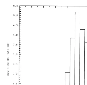
Fig. 6a,b presents the mean values of the collision efficiencies in a turbulent flow
Žcurve A and in calm air curve B as a function of the ratio of smaller droplet and. Ž .
droplet-collector radii. The drop-collector radius was 10 mm in Fig. 6a and 20 mm in Fig. 6b.
Fig. 7 shows a scattering diagram indicating the dependence of the collision
Ž .
efficiency normalized with respect to the pure gravity value on the interdrop relative
Ž
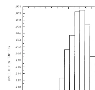
velocity normalized to the difference of drop terminal fall velocities induced by gravity. Fig. 8 presents the distribution of the collision efficiencies of 10- and 20-mm-radii droplets normalized with respect to the pure gravity value.
Fig. 5. Examples of the collision cross-sections for drop pairs containing 10- and 20-mm-radii droplets in
Ž . Ž .
different points of a turbulent flow shaded areas . The collision cross-sections in calm air pure gravity case are marked by small open circles. Large open circles are geometric cross-sections. The collision efficiencies Et
and E calculated for the cases of the turbulent flow and the pure gravity setting, respectively, are presented asg
Ž
Fig. 7. A scattering diagram indicating the dependence of the collision efficiency normalized to the pure
. Ž
gravity value on the interdrop relative velocity normalized with respect to the difference of drop terminal fall velocities induced by gravity.
Several conclusions can be drawn from the figures.
Ž .a The mean values of the collision efficiencies in case of a turbulent flow are higher than in the pure gravity case. The effect of turbulence increases with the decrease of the ratio of the radii of smaller droplets to drop-collector. The increase of the mean values of the collision efficiency in case of a 10-mm drop-collector significantly greater than in case of a 20-mm-radius drop-collector: it can be by factor of 5 to 9 as large as the
Ž .
corresponding values in the pure gravity case Fig. 6a . In case of 20-mm-radius drop-collector the mean collision efficiency is greater than corresponding gravity values by factor ranged from 1.2 to about 6, depending on the ratios of colliding droplet radii
ŽFig. 6b ..
Fig. 6. Mean values of collision efficiency as a function of the ratio of the radius of smaller droplet and the
Ž . Ž . Ž .
radius of the drop collector in a turbulent flow curve A and in calm air curve B . In a the radius of the
Ž .
Fig. 8. A distribution of the collision efficiencies of 10- and 20mm-radii droplets normalized with respect to the pure gravity value.
Ž .b The distribution of the collision efficiencies is rather wide. Comparably small changes of the interdrop relative velocity can lead to a significant increaseror decrease of the collision efficiency. The significant dispersion of the collision efficiency for the same absolute values of the interdrop velocities can be attributed to the fact that the collision efficiency largely depends not only on the magnitude of the interdrop relative velocity, but on the angles of droplet approach as well.
Ž .c In some cases drops are unable to collide collision efficiencies are equal to zeroŽ .
in spite of the fact that at the periphery of the area of drop hydrodynamic interaction
Ž .
drop approach takes place in Fig. 7, these cases are marked by symbols ‘‘zero’’ . Calculations show that the percent of cases with zero collision efficiencies varies from 0% to 20% of the total number of cases. The percent of these cases depends of the radii of interacting droplets.
The results show that the increase of the collision efficiency in a turbulent flow depends on the intensity of turbulence and on sizes of colliding droplets. We interpret
Ž .
The collision efficiencies in the pure gravity case grow rapidly with the drop size. For example, the collision efficiency of drops with radii 30 and 10 mm is as large as 0.5
ŽPruppacher and Klett, 1997 . As the values of the collision efficiency are limited to 1,.
an additional increase of the collision efficiency due to turbulence cannot be significant.
Ž
At the same time, the collision efficiency of small droplets of different radii say, 3
.
and 10 mm; 4 and 20 mm is about 0.02, so that a significant potential towards an increase of the collision efficiency can be supposed to be real. As it was shown by
Ž .
Pinsky et al. 1999a , small droplets tend to deviate from air stream lines in phase. Thus,
Ž .
the larger the difference in the droplet size inertia , the higher must be relative velocity induced by drop inertia and the higher must be the increase of the collision efficiency in
Ž .
a turbulent flow Fig. 6 .
Ž . Ž .
Effects of conclusions a and b on drop collisions will be discussed below in Section 4.
The mechanism leading to no collisions is discussed in Appendix C. Here we summarize the conclusions concerning the mechanism. Analysis shows that in the case
Ž
the ratio of the droplets fall velocities is less than a certain critical value which depends
.
on the ratio of particle masses , the interacting droplets form a tandem, in which droplets fall with the same velocities. The fall velocity of the tandem is greater than the velocity
Ž .
of a greater particle. In the case of two nearly equal particles drops the fall velocity of the tandem exceeds the velocity of each particle in the case of independent fall by about 50%. The increase of the fall velocity of the drop tandems increases their probability to collect other droplets. This possible effect requires special analysis. The formation of drop tandems can increase the probability of triple collisions.
The physical mechanism of the formation of such tandems involves in the interaction of velocity fields induced by the droplets during their fall. On the one hand, the difference in the terminal velocities due to gravity and the additional relative velocity
Ž
stemming from the drop inertia in case additional velocity increases the total interdrop
.
relative velocity favors the drop collision. On the other hand, the lowermost drop
Ž .
experiences acceleration by the flow induced by the upper one by the collector which favors droplet repulsion. This influence increases during the particle approach. In cases
Ž
of a comparably small ratio between droplet velocities at the infinity beyond the zone
.
of hydrodynamic interaction , both particles reach the same velocity at a certain separation distance and continue falling as a tandem.
4. Stochastic nature of drop collisions and its importance for cloud microphysics
In this section, we discuss the effects of stochastic processes on cloud microphysics. The main result of the paper is that in a turbulent flow interdrop relative velocities and collision efficiencies are random values with a wide dispersion. Hence, the collision kernels determining the probability of drop collisions are random values with a wide dispersion. If we take into account the fact that drop concentration fluctuations in a turbulent flow are determined by turbulent flow fluctuations, which are also random, all
Ž .
stochas-tic. Characteristic time and spatial scales of variations of all these microphysical values are determined by the properties of atmospheric turbulence and droplet size. For small cloud droplets a typical time scale is about 0.5 s and a typical spatial scale is one to few centimeters.
Thus, the process of collisions in a turbulent flow is highly inhomogeneous in space and in time. The question arises, what might be the effects of these inhomogeneities on the process of droplet collisions and other microphysical cloud properties.
Let us start the discussion with the fluctuations of droplet concentration. The droplet concentration inhomogeneity can by caused by many mechanisms. As it was shown in Section 1, the combined effect of turbulence and drop inertia can lead to the formation of drop concentration inhomogeneity. The spatial scales of these concentration fluctua-tions depend on the drop size. For small cloud droplets these scales equal one to few centimeters. The RMS amplitude of these fluctuations can amount to 30–40% of the
Ž . Ž .
mean concentration Pinsky et al. 1999a . Pinsky et al. 1998b found in a typical cumulus cloud the RMS amplitude of droplet fluctuation concentration to be 30% of the mean concentration. The probability of droplet collisions increases in these small volumes of enhanced concentration. Let us evaluate a potential effect of the droplet
Ž .
concentration fluctuations under assumption that these fluctuations do exist in clouds . As follows from the stochastic kinetic equation of collisions, the growth rate
Žfrequency of drop collisions is proportional to the multiplication of their concentrations.
n and n . Thus, the frequency of collisions increases in the areas of enhanced droplet1 2 concentration by a factor of 1.7 to 2. To evaluate the effect of these ‘‘subgrid’’ fluctuations of drop concentration on the collision rate averaged over large volumes of 107–1010 m3, typical of cloud model resolution, we have to evaluate the mean value of the multiplication n n . One can write:1 2
²n n1 2:s²n1:²n2:qRs s1 2
Ž
4.1.
²: 7 10 3
where symbol denotes averaging over a certain volume of the order of 10 –10 m ,
s1and s2 are the RMS values of drop concentration fluctuations, R is the correlation coefficient. In cloud models based on the stochastic kinetic equations of collisions the
² :² :
value n1 n2 is usually used. We can see that in case of positive correlation between drop concentration fluctuations, concentration inhomogeneity accelerates the collision
Ž . Ž .
process. This fact was discussed by Voloshuk and Sedunov 1975 , Kasper 1984 and
Ž . Ž . Ž .
Pinsky and Khain 1997b . According to Khain and Pinsky 1997 , Pinsky et al. 1999a ,
Ž .
small droplets with the radii 5 to 15 tend to concentrate in the same regions of a turbulent flow, so that the coefficient of correlation R is close to 1. Thus, from Eq.
Ž4.1 , the mean drop growth rate due to small droplet concentration the autoconversion. Ž .
rate increases by 10% to 15%. These evaluations are related to droplets, whose
Ž
concentration prevails and determines total droplet concentration 5- to 10 m
m-radii-.
droplets . Note, that droplets flux velocity divergence is proportional to the square of the
Ž .
Ž .
Pinsky and Khain 1997b assumed the existence of a ‘‘self-concentration’’ process of droplet collisions: larger cloud droplets being formed, tend to concentrate in certain volumes, where their concentration turns out to be much higher than the averaged concentration of such drops. The increase in the concentration of these droplets increases the probability of their collisions with the formation even larger droplets. These droplets, in their turn, tend to concentrate with even higher rate, etc. The main idea of the assumption is that the fast droplet spectrum broadening with formation of rain drops takes place in the regions, where the concentration of larger cloud droplets is much
Ž .
higher than the mean averaged concentration of such drops. In other areas the collisions of larger cloud droplets are too rare to form raindrops. This process was
Ž .
simulated by Pinsky and Khain 1997b using a simple model. A faster broadening of the ‘‘mean’’ spectrum was obtained, as compared to that of homogeneous droplet concentration. Further investigations are required to investigate the process.
The process of ‘‘self-concentration’’ can be very important in case of ice particles. It is known that ice particles’ concentration is highly inhomogeneous. High ice concentra-tions are observed in areas of enhanced turbulence. The process of collisions of drop and ice particles fields is a complicated problem. Note, however, that the simple evaluations presented above indicate the significance of the effect of the hydrometeors’ concentra-tion inhomogeneity on cloud evoluconcentra-tion.
Let us now evaluate the possible effects of turbulence on the collision kernel. The collision efficiencies between small cloud droplets in the pure gravity case are
Ž .
very small. It is generally accepted Jonas, 1996 that droplets must reach the radius of about 20 mm by diffusion to be able to grow further by collisions. In this case, the classical problem of cloud microphysics arises: the diffusion growth is unable to form
Ž .
wide droplet spectra in situ observed in cumulus clouds Brenguier, 1998 . The cloud droplet spectra contain significant concentrations of droplets with radii 30mm and even 40 mm in radii. For values of supersaturations typical of small cumulus clouds, it will
Ž .
take more than 1 h and a half for cloud droplets to reach the size Jonas, 1996 . The growth of drops by collisions to reach the rain drop size with the radii of several
Ž .
hundredmm will take one more hour Jonas, 1996 . It is known, however, that cumulus clouds of this type precipitate in a few tens of minutes after cloud formation. All hypotheses claiming to explain the drop spectral broadening at the stage of condensation growth are subject to uncertainty or contradiction. This situation was stated at the end of a many hours’ discussion taking place at a special session at the Conference on Cloud
Ž . Ž .
Physics, 17–21 August 1998 Everett, WA see, e.g., Brenguier, 1998 .
The increase of the collision efficiency in a turbulent flow may turn out to be crucial as concerns broadening of initially narrow droplet spectrum. The increase of the collision efficiency is especially pronounced for collisions of small cloud droplets with radii below 20mm. Such increase can reach a factor of 10 and even greater as compared to the pure gravity case, depending on the intensity of turbulence and size of drops in drop pairs.
To illustrate the effect of the mean increase of the collision efficiency on the drop size spectrum evolution, we solved the stochastic kinetic equation of collision. The
Ž .
my3. The initial spectrum was set narrow with the maximum at the 10-mm-radius. The initial size distribution corresponds to the droplet concentration of 300 cmy3. To exclude the possible influence of the ‘‘tail’’ of low concentration larger droplets, the size distribution was set equal to zero at the drop radii exceeding 20mm. The width of the initial spectrum is close to the width predicted by the adiabatic theory for the droplet
Ž
spectrum in cumulus cloud cores a few hundred meters above the cloud base Brenguier,
.
1998 . When simulating time development of the initial droplet size spectrum, the
Ž .
collision efficiencies of small droplets with the radii below 25mm were set four times as large as the pure gravity values. This factor of the collision efficiency increase corresponds to the results of calculations for comparably low intensity turbulence typical of the early cumulus clouds. Fig. 9a,b shows the drop size distributions after 4 min and 14 min of the simulation. To facilitate comparison, the size distributions in the pure gravity case are also shown. While in pure gravity case the maximum size of droplets at 12 min reached 22.5 mm, in case when turbulence effects are taken into account, the droplet size spectrum broadens rapidly with the formation of 33mm radius droplets. The droplet spectrum resulting in the turbulence case is in good agreement with in situ
Ž .
observed spectra in undiluted cores of cumulus clouds Fig. 2 in Brenguier, 1998 . The simulation of droplet size spectra evolution in this experiment continued up to 30
Ž .
min. The resulting spectra in the pure gravity case curve A and in the turbulent case
Žincrease of collision efficiency between droplets with the radii below 25mm. Žcurve B. Ž . Ž
at 30 min are shown in Fig. 10. In the figure the mass density function g ln a Berry
.
and Reinhardt, 1974 is used to characterize the drop size spectrum, which is related to
Ž . Ž . Ž .
the size distribution function f a as g ln a samf a , where m is the mass of a
droplet with radius a. One can see that in the pure gravity case the development of the drop size spectrum is very slow. At the same time, the turbulence effects on cloud droplet collisions being taken into account, the drop spectrum contains raindrops with radii of several hundred mm in 20–30 min. Thus, the stochastic effects induced by turbulence can be of crucial importance for the droplet spectrum development and rain formation.
Possible effects of random fluctuations of the collision efficiency and the collision kernel require special analysis. To evaluate the sensitivity of a size droplet spectra to random fluctuations of the collision kernel, we solved the stochastic kinetic equation of
Ž .
collisions for the Golovin kernel Voloshuk, 1984 , as well as for the geometrical
Ž .
collision kernel. The Golovin collision kernel is defined as Ksb m1qm , where m2 1 and m2 are the masses of colliding droplets, parameter b is usually assumed to be constant. In a general case, b is the function of time. To simulate effects of turbulence on the collision kernel fluctuations, parameterb was calculated as a random function of time obeying the log–normal distribution. The mean value was chosen equal to 1500
3 y1 y1 Ž .
cm g s Seesselberg et al., 1996 . The deviation determining the amplitude of
Ž .
Fig. 9. The droplet size distributions in the pure gravity case curve A and in case when the turbulence effects
Ž .
on the collision efficiencies of small cloud droplets is taken into account curve B at ts4 min. The initial y3 Ž .
spectrum reaches its maximum at the radii of 10mm, cloud water content is equal to 1 g m . b The same as
Ž .
Ž . Ž
Fig. 10. The same as in Fig. 9, but for ts30 min. In the figure, the mass density function g ln a Berry and
.
Reinhard, 1974 is used to characterize the drop size spectrum. One can see that in the pure gravity case the development of drop size spectrum is very slow. At the same time, the turbulence effects on cloud droplets collisions being taken into account, the drop spectrum contains rain drops as large as several hundred in radii.
kernel fluctuations was assumed thrice as large as the mean value. This value of deviation was derived as a first approximation from the results of calculations of the
Ž .
collision kernels in a turbulent flow. We generated 200 sets of random series of b t by
the Monte Carlo method. The droplet size distributions have been calculated for each set
Ž .
of b t using an analytical solution of the stochastic equation of collisions. Initial drop
size distribution was assumed exponential to permit the analytical solution. Cloud droplet content and concentrations were set the same as in the previous example.
Ž .
The size distributions obtained for each of the 200 sets of b t were averaged and the
mean drop-size distribution has been calculated at different times from 0 to 30 min. This averaged size distribution was compared to that obtained forb equal to the mean value. In case of bsconst, the maximal sizes of droplets radii were 32 and 65mm at ts10 and 20 min, respectively. In case of the collision kernel fluctuations the maximal values of droplet radii were 47 and 90mm, respectively. Note, however, that the increase of the
Ž .
A second attempt to check the sensitivity of droplet spectrum evolution to fluctua-tions of the collision kernel has been made using the geometrical collision kernel applied as a rule. The stochastic equation of collisions was solved by the method developed by
Ž .
Bott 1998 . Similar to the last example, the distribution of the collision kernel was assumed to be log–normal with deviations twice as large as the mean value. Different
Ž .
random sets K t were generated by the Monte Carlo method. The initial values ofg droplet concentration and cloud water content were the same as in the first example. The results of calculations support the conclusion reached using the Golovin kernel: fluctua-tions of the collision kernel favor the formation of larger droplets and the elongation of the tail of the droplet size spectrum. But as large collision kernels are rare, the number of these large droplets is too small to influence the modal radius of the droplet spectrum significantly. In some cases, random fluctuations of the collision kernel lead to remark-able acceleration of the droplet size spectrum broadening. However, in many other random series of the collision kernel fluctuations the effect was much lower. As a result, the drop size spectrum obtained by averaging over a great number of different realizations of the drop spectra evolution had actually the same modal drop radius as in case of the pure gravity geometrical collision kernel and long low concentration ‘‘tail’’ of larger droplets.
These preliminary evaluations show that the contribution of the mean increase of the collision efficiency and the collision kernel seems to prevail over the effects caused by random fluctuations of these values. This preliminary result needs, however, further analysis.
This conclusion, being supported by other investigations, could be of significant importance from the point of view of parameterization of turbulent effects on process of
Ž
collisions. If the effect of the mean increase of the collision efficiency the collision
.
kernel is dominating, the parameterization will be reduced to the multiplication of the pure gravity values by some factor depending on the drop size and intensity of turbulence.
Note that stochastic effects of turbulence are not necessarily caused by the inertia of cloud particles. For instance, drop concentration inhomogeneity arises during the entrainment of drop-free air into clouds through their boundaries.
The magnitudes and distributions of fluctuations of concentrations, the collision kernels, and relative velocities between particles are determined by the properties of cloud turbulence. As we mentioned above, turbulence in clouds is highly intermittent, so that the values of the dissipation rate are different in different regions of the flow. The approximation of cloud turbulence as isotropic is, possibly, too crude. This problem requires special investigation.
5. Conclusions
The collision efficiencies of small cloud droplets are calculated in a turbulent flow,
Ž
the velocity field of which was generated using a model of isotropic turbulence Pinsky
.
The results indicate that in a turbulent flow the collision efficiency is a random value
Ž .
with high dispersion. The collision efficiencies depend on the initial at the infinity interparticle velocities and angles of droplet approach. The mean values of the collision efficiency and the mean values of the collision kernel in a turbulent flow exceed the values measured or calculated for still air conditions. For instance, under turbulent intensity typical of early cumulus clouds, the mean values of the collision efficiency for a 10mm drop-collector are 5 to 9 times as large as the values in the pure gravity case. In case of a 20-mm-radius drop-collector the mean collision efficiencies are greater than the corresponding gravity values by a factor ranging from 1.2 to about 6, depending on the size ratios of colliding droplets.
The collision efficiencies in a turbulent flow are shown to be very sensitive to relative
Ž .
droplet velocities. Even a small variation of about 10% of the interdrop relative velocity can result in values of the collision efficiencies twice as large as in the calm air. According to Fig. 7, the collision efficiency tends to decrease with the increase of normalized relative interdrop velocity. Note that this tendency was observed for particular drop mass ratios and usually under small droplet collectors. For other cases, for instance, for a drop pair of 30 and 15mm, a pronounced positive correlation between
Ž .
the collision efficiency and the interdrop relative velocity at infinity was observed. Analysis of mechanisms leading to a negative or positive correlation is beyond the frame of this study and needs special consideration.
In numerical experiments, on drop collisions within a turbulent flow a new effect was discovered, namely, in some cases the collision efficiencies in a turbulent flow appeared
Ž .
to be equal to zero no collisions . We analyze this effect for a simple case of
Ž .
gravitational vertical fall of particles along the axis connecting their centers. Analysis shows that in this case the ratio of the droplets fall velocities is less than a certain
Ž .
critical value which depends on the ratio of particle sizes the falling particles form a tandem, in which particles fall with the same velocities. We attribute the effect to the fact that a flow field induced by a drop-collector tends to push away the other droplet in the pair. Note that in this simplified case of drop approach along the vertical axis, drops form a stable ‘‘tandem’’ falling with a sedimentation velocity exceeding the terminal velocity of each droplet in the pair.
Statistical estimations obtained for the turbulent flow model show that the number of interactions with zero collision efficiency varies within 0% and 20% of all interactions, so that the existence of zero collision efficiencies has a relatively small effect on the mean values. It is possible, however, that in cases of interaction of small particles of different densities the fraction of cases with no collisions might be greater. For example, the collision efficiencies of comparably small crystals with sizes of several tens ofmm
Ž
and cloud droplets with the radii less than 20 mm are equal to zero Pruppacher and
.
Klett, 1997 . We suppose that these zero values of the collision efficiencies can be rationalized in a way similar to that analyzed in the paper. On the other hand, the distribution of interparticle relative velocities means that in some cases, when collisions in the pure gravity case are forbidden, there is a non-zero probability of their collisions in a turbulent flow.
inhomo-geneity accelerates the rate of droplet collisions, which are effective in the areas of increased droplet concentration. By solving the stochastic kinetic equation of collisions, it was shown that the increase of the collision efficiency of small cloud droplets controls the broadening of the initially narrow droplet size spectrum and accelerates the process of rain formation. The results indicate that the increase of the collision efficiency of small cloud droplets in a turbulent flow can, probably, be regarded as the mechanism responsible for the in-situ observed broadening of droplet spectra in undiluted cores of
Ž .
cumulus clouds Brenguier, 1998 .
Preliminary evaluations of the effects of random fluctuations of the collision effi-ciency and the collision kernel in a turbulent flow indicate that these fluctuations favor the formation of a low concentration large drops ‘‘tail’’ in the drop-size spectrum. However, the concentration of the large droplets turned out to be too small and failed to change the droplet spectrum. The effect requires further investigation. This conclusion could be of significant importance from point of view of parameterization of turbulent effects on the process of collisions. If the effect of the mean increase of the collision
Ž .
efficiency the collision kernel is dominating, parameterization will be reduced to the multiplication of the pure gravity values by some factor depending on the drop size and intensity of turbulence.
Summing up, we would like to note, that we do not clime to use the distributions of the collision efficiencies obtained in this study for purposes of parameterizing turbulent effects. It is connected with some limitations of the model of turbulent flow used in calculations. First, the turbulent model is two-dimensional. Second, the model is a model of isotropic turbulence. Atmospheric turbulence, particularly in clouds, is highly inter-mittent with wide range fluctuations of the dissipation rate. We assume that the intermittence plays a significant role in drop motion and interaction. Besides, the model used in the calculations has no time variations. Incorporation of time dependence of turbulent velocity into the model can influence the results. In this connection we
Ž .
mention the study by Zhou et al. 1998 investigating the role of turbulence on the collision kernel using a turbulent model based on the solution of the Navier–Stokes equation. A significant increase of the collision kernel has been found in case of time
Ž
independent velocity field the velocity field obtained in the model was ‘‘frozen’’ at a
.
certain time instance . However, the utilization of the velocity field evolving with time instead of the ‘‘frozen’’ velocity field resulted in a 20% decrease of the collision kernel as compared to the time-dependent case. On the whole, we qualify the results as just preliminary. The problem of creating a time-dependent turbulent model, that will be able to describe the turbulence structure at high Reynolds numbers, and the calculation of the collision efficiency distributions using such a model is very complicated and requires further investigation.
Acknowledgements
Ž
This study was partially supported by the Germany–Israel Science Foundation grant
.
0407-008.08r95 , and by the Israel Science Foundation founded by the Israel Academy
Ž .
Appendix A. The model of isotropic turbulence
Our analysis of drop interaction and collisions in a turbulent flow is based on the
Ž .
model of isotropic turbulence described by Pinsky and Khain 1995, 1996 in detail. Below we present a brief description of the model.
The turbulent model generates different realizations of a turbulent flow with given correlation and spectral properties. The components of the velocity field are calculated as the sum of a large number of harmonics with a set of wave numbers lk and random
Ž
amplitudes. In contrast to other models of this type e.g., Kraichnan, 1970; Maxey,
.
1987 , in our model for each wave numberlk is described by a set of random harmonics
Ž .
with different directions of the wave vector angles wm . The velocity field is character-ized by the continuity, isotropy, and homogeneity properties.
The longitudinal structure function for the turbulent velocity field, suggested by
Ž .
Batchelor Monin and Yaglom, 1975, p. 408 , has been chosen for the description of a locally isotropic turbulence in the inertial and viscous turbulence ranges:
y2r3
X X2 X2
DLL
Ž .
r s2GrŽ
1qFr.
,Ž
A.1.
Ž .y1 Ž .y3r2 1r2
where Gs´ 30 n and Fs 15Cn ´ . Here ´ is the dissipation rate of turbulent kinetic energy, n is the kinematic viscosity of air, and Cs2 is a non-dimen-sional constant. This approximation formula follows asymptotic behavior of the structure function in far viscous and far inertial ranges corresponding to Kolmogorov’s theory
Žsee, Monin and Yaglom, 1975 . It is also simple enough for analytical calculations. The. Ž .
longitudinal structure function A.1 has the following asymptotes:
y1 X2 X
is the Kolmogorov microscale and L is the external turbulence
o o
Ž .
scale where velocity fluctuations become non-isotropic . In the model presented,´ and
L are external parameters.o
The suggested model generates two-dimensional isotropic velocity fields having the
Ž .
longitudinal structure function A.1 of 3-D turbulence. Thus, the model generates velocity fields having properties of 3-D turbulence. For example, the energy spectrum in
Ž .
the inertial range will be the y5r3 Kolmogorov spectrum. Some characteristics of the turbulent flow model used for simulations are the following:
Dissipation rate´ 100 cm2 sy3
Minimum wave number 0.06 my1
Maximum wave number 800 my1
Number of harmonics lk 57
Number of angles wm for each harmonic 120 Number of random values used for velocity field formation 13 680