this PDF file CAPACITY FACTOR BASED COST MODELS FOR BUILDINGS OF VARIOUS FUNCTIONS | Wibowo | Civil Engineering Dimension 2 PB

CAPACITY FACTOR BASED COST MODELS FOR BUILDINGS OF

VARIOUS FUNCTIONS

Andreas Wibowo

Researcher, Research Center for Human Settlements, Ministry of Public Works Lecturer, Graduate Program in Civil Engineering, Parahyangan Catholic University

Email: andreaswibowo1@yahoo.de

Wahyu Wuryanti

Researcher, Research Center for Human Settlements, Ministry of Public Works Email: wuryanti@bdg.centrin.net.id

ABSTRACT

The desired accuracy level of an estimate heavily relies on the availability of data and information at the time of preparing the estimate. However, an estimate often must be made when data and information are not complete. At earlier stages of project implementation at which data and information are minimal, a client is often required to prepare a cost estimate. This paper discusses the capacity factor-based cost models for buildings with total areas serving as the proxy of capacity. A total of four cost models for different building functions are presented in this paper. Based on the models, most building functions with the exception of housings, exhibit decreasing return to scale, meaning that the unit measure of cost expressed by cost per square meter declines as the size of capacity increases. The cost models are then applied to estimate the development unit cost for different demographical unit measures.

Keywords: cost estimation, order-of-magnitude estimate, capacity factor, regression analysis.

INTRODUCTION

Cost estimation is one of the critical steps to the success of a construction project implementation. Based on the estimate, strategic decisions are made, starting from the decision on bringing or not bringing the project into realization, the determina-tion of construcdetermina-tion materials and methods, the selection of contract type, the procurement of construction contractor, and so forth. The accuracy is thus becoming the keyword to every single estimate prepared because the estimate should lead the decision maker to the correct conclusions to make best decisions.

US National Estimating Society defines the cost estimation as the art of approximating of possible cost amounts required to complete a task based on the availability of information at the time of preparing the estimate [1]. When referring to the definition, there are two issues to address. First, estimation is more viewed as art than science. This might reflect that the resulting estimation will be dependent on who prepares and whom it is prepared for.

Note: Discussion is expected before November, 1st 2007, and will be published in the “Civil Engineering Dimension” volume 10, number 1, March 2008.

Received 4 January 2007; revised 29 March 2007; accepted 20 April 2007.

Cost estimation made by one cost engineer should not necessarily be the same with that of another cost engineer because of different relative experiences, perspectives and assumptions of estimation, knowledge, organizations with which they work.

Second, the availability of information at the time of preparing the estimate is influential. It has been widely acknowledged that the successful mate-rialization of a construction project is exposed to many internal and external factors and this characteristic is inherent to any construction project. The availability of proper data and information is thus essential to identifying, analyzing, and anticipating risk and uncertainty factors at earlier stages to minimize any possible deviations from estimates. The more appropriate data and informa-tion, the more accurate the estimate should be.

in many literatures as the order-of-magnitude esti-mate (OME) or conceptual screening estiesti-mate. The issue is how to improve the accurateness of OME under minimal data and information conditions by making use the historical project data. This will be central to this paper.

ORDER OF MAGNITUDE ESTIMATE

Several classifications on cost estimate can be found in literatures. American Association of Cost Engi-neers (AACE) [2], for instance, categorizes cost estimate into three groups, as presented in Table 1. One interesting feature of Table 1 is the asymme-trical accuracy range. It has a longer tail in the positive direction than the negative one, suggesting that a very high cost overrun is potential while a cost underrun is limited. For small projects, cost escalation in the order of 10- 20% is common but for larger projects with longer duration, the limit is the sky [3]. The escalation can be attributed to inefficien-cy, inflation, information characteristic flow, change of contract, and type of contract. Table 1 also pre-sents the accuracy range as the function of the project progress; the accuracy increases with the project maturity. Another classification system groups cost estimate by their accuracy: level one when it ranges from -10 to +40%, level two from –5 to +25% and level three from –3 to +10% [4].

Table 1 AACE Estimation Classification and Me-thods [2]

Semi detailed 30 to 50 Square foot, Parametric

or Elemental

Definitive -5 to +15 Engineer’s Bid,

Detailed

Over 60 Detailed pricing and

takeoff

Cost of Preparing Estimate

The cost of preparing an estimate depends on the desired level of accuracy and the availability of data and information at the time of preparing the estimate. The manual estimation cost to generate the accuracy of -5 to +15% can be as high as 25 to 30 times of the manual cost of estimation to produce the accuracy of -30 to +50%. The introduction of cost estimating software allows the cost of estimation to be reduced but the factor remains at five or more, as shown in Table 2 [5]. Table 2 also shows that the cost of preparing an estimate depends on the size of project.

Table 2. Cost of Estimation (in Thousand USD) [5]

Cost of Project in Million USD Estimate Type Accuracy

range (%) Less than 1.0 1.0 to 5.0 5.0 to 50.0

(1) (2) (3) (4) (5)

Order of magnitude -30 to +50 7.5 to 20 17.5 to 45 30 to 60

Budget -15 to +30 20 to 50 45 to 85 70 to 130

Definitive -5 to +15 35 to 85 85 to 175 150 to 330

Level of Influence of Estimate

It is not elusive when OME has the widest range of accuracy if compared to other estimating methods. Nevertheless, the OME method has also the highest level of influence on project cost. At the very beginning of the project lifecycle, the OME has a 100% influence on the next project cost because it can result in a go/no-go decision. This signifies the importance of the OME. Given that the project is prolonged, it steps into the next stage while information available to the cost engineer accumu-lates. Having more information, the cost engineer is now able to select the most appropriate construction methods, technologies, materials of the project and estimate their cost. At this stage the influence of an estimate on the project cost decreases. As the project goes further and becomes mature, the influence lessens and finally disappears when the project is successfully completed.

Capacity Factor Based Estimate

One of the most widely-used OME methods in manufacturing and petrochemical industries is the capacity factor method. The method estimates the cost of a new facility at the desired size of capacity based on the known cost of similar facility at different capacity level using the following formula:

m

estimated cost. The coefficient m depends on the type of industry. In petrochemical industries, for example,

m is normally taken as 0.6 so that the method is also known as the six-tenths factor rule although the seven-tenth factor rule is also recommended for some instances [5]. The cost models developed in this study are based on the capacity factor method. The target is to determine the coefficient m that holds for building construction.

DATA COLLECTION AND ANALYSIS

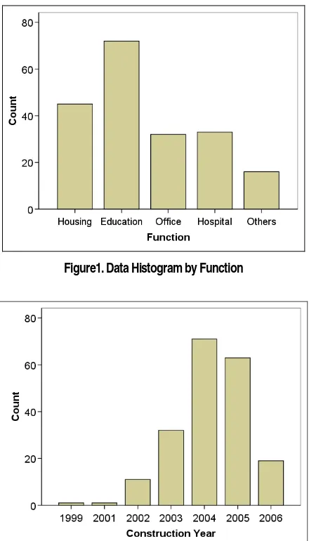
Figure1. Data Histogram by Function

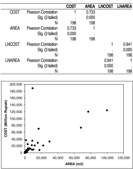
Figure 2. Data Histogram by Construction Year

Because data sets are collected from different years and locations, they must be adjusted to the same basis; namely year 2006 and Bandung City. The adjustment process is sometimes known as data normalization. The study employs the consumer price index (CPI) published by the Central Statistic Bureau for normalizing data sets. The use of CPI is not without problem anyway because the index is based on prices of general goods and services, not specifically based on construction associated mate-rials and wages. In this sense the construction cost index (CCI) rather than general CPI is obviously more robust. However, it is confronted with the fact that no official CCI has been available. The authors therefore conclude that the use of CPI for data correction is optimal in today’s situation when taking their advantages and disadvantages into considera-tion. In the future the development and the use of CCI should be encouraged and envisaged.

The formula used for data normalization is written as follows [6]:

X B

A Y

X B A Y

CPI

CPI

C

C

=

(2)

Where

C

_YAis the cost in year Y at location A;

A Y

CPI

, CPI in year Y at location A;

C

_BX, cost at

location B in year X;

CPI

_BX, and CPI at location B

in year X.

Descriptive Analysis of Unit Cost

After normalizing data, the next step is to examine the distribution of the normalized data. Data examination allows the researcher to attain a basic understanding of the data and relationships between the variables [7]. The first data to examine is the unit measure of cost expressed as cost per square meter. Table 3 lists the statistics of descriptive analysis on the unit cost. As shown, the unit cost ranges from Rp. 1.52 million per m2 _{to Rp. 2.34}

million per m2 _{at the 95% confidence level with the}

mean computed at about Rp. 1.93 million per m2_{. If}

five percent highest and lowest values are elimi-nated, the trimmed mean equals to Rp. 1.52 million per m2_{. The decrease may indicate that a number of}

extremely-high data substantially influence the overall data structure. If these data are ignored, the resulting mean shifts to the negative direction. The high skewness of 7.125 strongly indicates that unit cost is far from being normally distributed; it is potentially distributed to higher values. This statistic might be associated with the high standard deviation relative to the mean which asserts that the unit cost is highly dispersed

Table 3. Descriptive Statistics of Unit Cost of Gene-ral Buildings

Statistic Std. Error

Mean 1,929,105 208,184

95% Confidence Interval for Mean Lower Bound 1,518,550

Upper Bound 2,339,660

5% Trimmed Mean 1,521,550

Median 1,446,486

Variance 8,581,418,543

Std. Deviation 2,929,406

Minimum 150,127

Maximum 28,914,036

Range 28,763,909

Interquartile Range 791,775

Skewness 7.125 0.173

Kurtosis 56.029 0.344

Table 4a. Kruskal Wallis Non-Parametric Test

Function N Mean Rank

Unit Cost (Rp/m2) Housing 45 59.24 Education 72 88.14 Office 32 143.38 Hospital 33 124.55

Others 16 124.44

Total 198

Table 4b. Test Statistics

Unit Cost b. Grouping Variable: Function

Area as the Proxy of Capacity

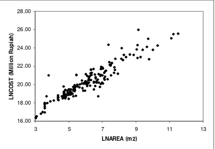
The data examination through univariate analysis is carried on total area coded as AREA and project cost coded as COST with descriptive statistics listed in Table 5. The regression analysis is engaged to obtain the mathematical relationship between AREA as the independent variable and COST as the dependent variable. However, there exists a precondition to meet prior to undertaking the regression analysis. The regression analysis requires the conditional variance of the dependent variable to be constant irrespective of independent variable (the assumption of homoscedasticity). While this requirement is only satisfied when the data distribution is normal [9], the normality of variables must be tested. For this reason, the Kolmogorov-Smirnov (K-S) test [8, 9] is conducted with the results shown in Table 6.

Table 5. Descriptive of Total Areas and Costs

Variable N Minimum Maximum Mean Std. Deviation

Skewne ss

(1) (2) (3) (4) (5) (6) (7)

COST (thousand Rupiah)

198 12,199 187,576,706 5,129,958 19,862,984 6.525

AREA (m2_{) 198 21 100,000 2,649 10,646 7.035}

Valid N (listwise) 198

When examining the statistics in Table 5, both

COST and AREA have a very high skew, indicating that being normally distributed is unlikely for data of the variables. The statistic Z in Table 6 columns 1 and 2 affirms that the normality assumption for both variables is indeed statistically rejected at the 0.05 significance level. Hence, the requirement is not fulfilled.

In statistical analysis, data transformation is some-times considered necessary to correct violations of statistical assumptions and/or improve relationship between variables [7]. Data transformation by taking the natural logarithm of variable values is

performed in this study to make their distribution closer to normal:

LNCOST = ln (COST) (3)

LNAREA = ln (AREA) (4)

Table 6. One-Sample Kolmogorov-Smirnov Test

Statistics COST AREA LNCOST LNAREA

(1) (2) (4) (3)

N 198 198 198 198

Normal Parameters Mean 1,929,105 2,649 20.0985 5.9194

Std. Deviation 2,929,406 10,646 1.86973 1.69748

Most Extreme Differences

Absolute 0.300 0.402 0.090 0.083

Positive 0.300 0.398 0.090 0.083

Negative -0.294 -0.402 -0.067 -0.054

Kolmogorov-Smirnov Z

4.225 5.664 1.265 1.162

Asymp. Sig. (2-tailed)

0.000 0.000 0.081 0.134

Note

a. Test distribution is Normal. b. Calculated from data.

As expected, the statistic Z in Table 6 (see columns 3 and 4) explains that normal distribution assumption is accepted at the 0.05 significance level. The correla-tion coefficient also improves substantially from 0.733 to 0.941, as shown in Table 7. Figs. 3a and 3b exhibit the correlation between two variables before and after transformation, respectively. As shown, substantial improvement in terms of correlation has been made as a result of data transformation.

Table 7. Pearson Correlation Between Original and Transformed Variables

COST AREA LNCOST LNAREA

COST Pearson Correlation 1 0.733

Sig. (2-tailed) . 0.000

N 198 198

AREA Pearson Correlation 0.733 1

Sig. (2-tailed) 0.000 .

N 198 198

LNCOST Pearson Correlation 1 0.941

Sig. (2-tailed) . 0.000

N 198 198

LNAREA Pearson Correlation 0.941 1

Sig. (2-tailed) 0.000 .

0 20,000 40,000 60,000 80,000 100,000 120,000

AREA (m2)

16.00

Figure 3b. Scattergram of Cost and Area on Log-Log Paper

COST MODELS DEVELOPMENT

The regression analysis employed in this study results in statistics as shown in Tables 7a-7c. The coefficient of determination is very high (0.884), implying that 88.4% variance in dependent variables can be explained by the regression model. The analysis of variance (ANOVA) also suggests that the model is statistically significant at the 0.05 level. Based on the regression coefficients, the following linear cost model can be established:

LNCOST = 1.036×LNAREA + 13.966 (5) Eq. (5) can be simply rewritten as

LNCOST = LNAREA1.036 _{+ ln(1,162,403) (6a)} 13.966 and standard deviation 0.636 (see Table 7a). If the estimate is not expressed as a single value but rather a range value, the range cost model will be:

LNCOST = 1.036×LNAREA + 13.966 +

0.636×Φ-1₍α_{) (7a)}

Where Φ-1₍α_{) is the inverse of cumulative}

distribu-tion funcdistribu-tion of standard normal distribudistribu-tion, α, the probability of being less than computed value. The values of Φ(α) are available in most statistics textbooks and standard spreadsheet software. If the lower and upper limits of estimates are taken, respectively, as the 5th _{percentile level or there would}

be a 95% chance of it being exceeded and the 95th

percentile level that has a five percent probability of being exceeded, Eq. (7a) can be reformulated as:

LNCOST = 1.036×LNAREA + 13.966 ±

0.636× 1.645 (7b)

Similarly, taking the inverse of the natural loga-rithm of variables yields:

COST = (409,334 to 3,300,922) ×AREA1.036 _(7c)

Based on Eq. (7c), it is trivial to see that there is a 90% confidence level of estimates falling into the range.

Table 7a. Linear Regression: Model Summary

Model R R Square Adjusted R Square Std. Error of the Estimate

1 0.941 0.885 0.884 0.636

Note

a. Predictors: (Constant), LNAREA b. Dependent Variable: LNCOST

Tabel 7b. Regresi Linear: ANOVA

Model Sum of Squares df Mean Square F Sig.

1 Regression 609.308 1 609.308 1504.378 0.000

Residual 79.385 196 0.405

Total 688.693 197

Note

a. Predictors: (Constant), LNAREA b. Dependent Variable: LNCOST

Tabel 7c. Regresi Linear: Coefficients

Unstandardized Coefficients

Standardized Coefficients

t Sig.

Model B Std. Error Beta

1 (Constant) 13.966 0.164 84.919 0.000

LNAREA 1.036 0.027 0.941 38.786 0.000

Note

a. Dependent Variable: LNCOST

Cost Models by Function

Applying the similar procedure, the cost models for different functions are derived. Due to limited length of the paper, this paper only discusses the model, not detailed statistics (detail can be found in [6]). As can be seen in Table 8, all models are significant at the 0.05 level and have satisfactory determination coefficients with computed R2 _{above 0.70.}

Table 8. Summary of Cost Models by Functions

Model R2 _Sig.

Function

Single Estimate Range Estimate

(1) (2) (3) (4) (5)

a. Range estimate is based on the 90% confidence level

b. _{No differentiation is made for educational buildings. A further classification}

(e.g., elementary schools, junior high schools, and senior high schools) causes size of samples insufficient for statistical analysis.

Capacity Factors

Let C2 and Q2 be respectively the project cost and the

size of capacity (area) of a facility. Using Eq. (6c), the following relationship must hold:

C2 = 1,162,403×Q21.036 (8)

If there is another facility constructed at cost C1 with

a capacity of Q1, using the similar Eq. (6), the

C1 = 1,162,403×Q11.036 (9)

Eq. (10) is nothing other than the capacity factor-based cost model for general building construction with m being equal to 1.036. The similar procedures can also be taken to derive the cost models for different building functions. Subsequently, Eq. (1) can be rewritten as:

1

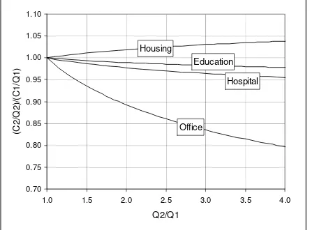
condition is called as the increasing return to scale. If the opposite is the case or m is smaller than unity, the decreasing return to scale takes place; implying that the higher the size of capacity, the lower the cost per unit capacity. Referring to the cost models in Table 8, all functions but housings exhibit decreasing return to scale. For instance, the increase in the total area by four times can reduce the cost per m2 _{by a}

factor of 0.8 for office buildings. Fig.4 depicts how the unit measures of cost of buildings change when the size of capacity increases. One reason that might explain the existence of decreasing return to scale could be associated with the layout of building. It is very common that the size of the communal facilities, public, and shared rooms with minimal wall partitions is substantial relative to the total area of building for general offices or public buildings.

Housing

Figure 4. Impact of Increase in Total Area on Unit Measure of Cost

Unit Measure of Development Cost

The formulas given in Table 8 can also be used for estimating the unit measure of development cost (in many respects the development cost is similar to the

program cost at public institutions). For instance, based on the Guideline on Urban Environmental Planning [10] one regional hospital is required per 240,000 inhabitants. Under the assumption that three beds are needed for every 1,000 inhabitants and every bed requires a gross area of 30m2 _{[11], the}

total area of one unit regional hospital equals to 21,600m2 _{(240,000/1,000×3×30). Based on this}

information, the project cost will be in the range of Rp. 20.91 billion and Rp. 39.39 billion, with the average cost computed at Rp. 28.70 billion.

As for educational buildings, the Guideline states that for every 4,800 inhabitants, one unit junior high school (Sekolah Lanjutan Tingkat Pertama or SLTP) is required. A standard SLTP building school has six class rooms, each of which is designed to accommodate 30 students so that each school is occupied by 180 students. If the gross area for each occupational unit is estimated to be 10m2 _per

student [11], the total area of one unit standard SLTP building equals to 1,800m2_{. The estimated}

project cost will be Rp 2.24 billion or, if expressed in the range estimate, the cost will be between Rp 1.11 billion and Rp. 4.41 billion per 4,800 inhabitants. Table 9 provides the more detailed estimated development unit costs for educational buildings, offices, and hospitals.

Table 9. Estimated Development Cost Unit

Estimated Cost (in billion Rupiah)

Function Number of

Inhabitants

to Serve Mean Lower Limit

Elementary 1,600 2.09 1.04 4.12 1,306

Junior Hi-School 4,800 2.24 1.11 4.41 466

Educational buildings

Senior Hi-School 4,800 2.24 1.11 4.41 466

Kecamatan

(subdistrict)

120,000 10.28 3.22 32.86 86

Wilayah (district) 480,000 19.78 6.19 63.21 41 Public offices

City 1,000,000 37.41 11.71 119.54 37

Hospitals Wilayah (district) 240,000 28.70 20.91 39.39 120

Note

a. Lower and upper limits are determined based on the 90% confidence level b. CPR = cost per inhabitant

Comparative Study on Capacity Factors

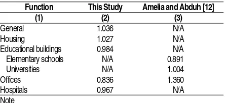
demonstrate the opposite. Table 10 presents in more details the results of two studies. No further com-ments could be made since the data of the referenced work [12] were not published.

Table 10. Comparative Study on Capacity Factors

Function This Study Amelia and Abduh [12]

(1) (2) (3)

General 1.036 N/A

Housing 1.027 N/A

Educational buildings 0.984 N/A Elementary schools N/A 0.891

Universities N/A 1.004

Offices 0.836 1.360

Hospitals 0.967 N/A

Note

N/A = not available

CONCLUSION AND RECOMMENDATION

The desired accuracy level of an estimate heavily relies on the availability of data and information at the time of preparing the estimate. However, the ideal situation where the cost engineer is equipped with complete and detailed data and information is not always encountered. An estimate must often be prepared with minimal data and this commonly happens during the early stage of project life cycle. This paper discusses the Order of Magnitude Estimate (OME) modeling based on capacity factors with area serving as the proxy of capacity. The cost models for different building functions are presented in this paper. The study also reveals that most building functions except housings, exhibit the so-called decreasing return to scale. It means that an increase in the size of capacity reduces the cost per unit capacity. The models are also applied to estimate the development cost unit based on certain demographical unit measures.

This research can be further developed by incur-porating some factors not accommodated in the models presented. The number of floors or the type of structure, for instance, can be integrated into the models as controlling factor so that the resulting models will be quasi-parametric. There exist many avenues open to further research. However, any research on construction cost estimation requires extensive historical project cost data. The colla-boration and cooperation with all stakeholders of the construction industry are sought to foster research activities on cost estimation in Indonesia that will benefit both academicians and industry practitio-ners.

REFERENCES

1. Soeharto, I., Manajemen Proyek: Dari Konsep-tual sampai Operasional, first edition, Penerbit Erlangga, Jakarta, 1995.

2. Ahuja H.N., et al., Project Management: Techni-ques in Planning and Controlling Construction Projects, second edition, John Wiley&Sons, New York, 1994.

3. Harrison F.L., Advanced Project Management, second edition, Gower Publishing Company, Hants, 1985.

4. Peurifoy, R.L., and Oberlender, G.D., Estimating Construction Costs, forth edition, McGraw-Hill, New York, 1989.

5. Nelson H.C., et al., Capital Investment Cost Estimation in Humpreys, K.K. (Ed.),Jelen’s Cost and Optimization Engineering, third edition, McGraw-Hill, 1991.

6. Puslitbangkim, Estimasi Biaya Satuan Pem-bangunan Bidang Permukiman, Final Report, Bandung, 2006.

7. Phaobunjong, K., and Popescu, C.M., Parametric Cost Estimating Model for Buildings, AACE International Transaction, 2003 <www.aacei. org>.

8. Devore, J.L., Probability and Statistics for Engi-neering and the Sciences, second edition, Thomas Nelson Australia, Melbourne, 1987.

9. Ang, A.H-S and Tang, W.H., Probability Con-cepts in Engineering Planning and Design, John Wiley&Sons, New York, 1978.

10. Ministry of Public Works, Pedoman Perencana-an LingkungPerencana-an PermukimPerencana-an Kota, third edition, Ministry of Public Works, Jakarta, 1983.

11. Juwana, J.S., Panduan Sistem Bangunan Ting-gi, first edition, Penerbit Erlangga, Jakarta, 2005.