Nihonjin eigo gakushusha ni totte no eigo /r/ to /l/ no konnando : onkyo bunseki ni yoru

Title Sub Title Author Publisher Publication year Jtitle Abstract. Notes Genre URL. Powered by TCPDF (www.tcpdf.org). Difficulty levels of English /r/ and /l/ for Japanese learners : an acoustic analysis 日本人英語学習者にとっての英語/r/と/l/の困難度 : 音響分析による 北川, 彩(Kitagawa, Aya) 慶應義塾大学外国語教育研究センター 2016 慶應義塾外国語教育研究 (Journal of foreign language education). Vol.13, (2016. ) ,p.21- 42 The present study aimed to examine phonetic and phonological learning with a specific focus on production of /r/ and /l/ and to identify the difficulty level of these approximants by defining /r/ and /l/ as easy, learnable or difficult items for Japanese learners of English. Acoustic analyses were conducted, where the third formant was measured for /r/ and /l/. The variables obtained from the analyses were submitted to three statistical tests, a cluster analysis, a multivariate analysis of variance and a discriminant analysis. The results showed that both approximants were difficult for Japanese learners to learn to produce. Despite the difficulty in learning them, it was also found that there was an individual preference about which approximant was learned faster. Some Japanese learners of English were learning /r/ faster than /l/ whereas others were learning /l/ faster than /r/. Further studies will be required to explore what creates these individual differences, and how positively the preference for learning /r/ or /l/ can affect the learning of both approximants. 研究論文 Departmental Bulletin Paper http://koara.lib.keio.ac.jp/xoonips/modules/xoonips/detail.php?koara_id=AA1204 3414-20160000-0021.

Difficulty levels of English  and  for Japanese learners: An acoustic analysis. Difficulty levels of English  and  for Japanese learners: An acoustic analysis Aya Kitagawa Abstract The present study aimed to examine phonetic and phonological learning with a specific focus on production of  and  and to identify the difficulty level of these approximants by defining  and  as easy, learnable or difficult items for Japanese learners of English. Acoustic analyses were conducted, where the third formant was measured for  and . The variables obtained from the analyses were submitted to three statistical tests, a cluster analysis, a multivariate analysis of variance and a discriminant analysis. The results showed that both approximants were difficult for Japanese learners to learn to produce. Despite the difficulty in learning them, it was also found that there was an individual preference about which approximant was learned faster. Some Japanese learners of English were learning  faster than  whereas others were learning  faster than . Further studies will be required to explore what creates these individual differences, and how positively the preference for learning  or  can affect the learning of both approximants.. 1. Introduction 1.1 Purpose of the study. Previous studies have pointed out the difficulty of Japanese learners learning to perceive and produce English  and  (Flege, Guion, Akahane-Yamada, & Yamada, 2004; Goto, 1971; Yamada, 1995). This is partly because of the difference in the phonological inventory of approximants between the two languages: English has four voiced approximants, , whereas Japanese has only two approximants, . Japanese does not have a voiced alveolar approximant, , and a voiced alveolar lateral approximant, , unlike English (English  should be transcribed as  if based on IPA, but  will be used in this paper following the conventional transcription).. 21.

慶應義塾 外国語教育研究 第13号. It should also be noted that although previous research often has found that Japanese learners of English tend to perceive and produce the English syllable-initial  and  as Japanese , English  and Japanese  are phonetically different. Japanese  is not even classified as an approximant. It is a flap, labelled as  or , which is articulated with a brief closure immediately before the following sound by quickly contacting the tip of the tongue with the alveolar ridge (Kent & Read, 2002). It rather sounds similar to an English flap used in American English, as in better. Japanese  and English  thus have very different phonetic qualities. The contrastive phonetics and phonology above suggest that Japanese learners of English, less experienced learners in particular, would have difficulty in producing  and  in a native-like manner. There seems to be a lack of consensus as to which approximants are more likely to be learned, however, especially concerning production. Some argued that  was learned with more ease (Aoyama et al., 2004; Hazan, Sennema, Iba, & Faulkner, 2005), while others maintained that both could be equally learned (Flege, Takagi, & Mann, 1995; Slawinski, 1999). This study therefore analyzed the production of these two approximants by Japanese learners with no experience of living in an English-speaking country, using acoustic analyses, in order to define the level of difficulty for these approximants. 1.2 Learning of L2  and . The difficulty of discriminating perceptually between English  and  for Japanese learners was empirically examined (Goto, 1971; Hallé, Best, & Levitt, 1999; Yamada, 1995). Goto (1971) conducted an experiment, where American and Japanese participants read a list of words including  and  tokens, and then identified the tokens as  and  by listening to their own recorded samples or the other participants’. He found that both proficient and less proficient Japanese participants discriminated between  and  in perception poorly. Yamada (1995) is in accordance with Goto (1971), but claimed that the experience of living in the U.S. affected accuracy in perceiving these approximants. Whereas the findings of Guion, Flege, Akahane-Yamada, and Pruitt (2000) showed that no Japanese sounds, including vowels and consonants, were similar to  and  perceptually, they reported that  was closer to , a Japanese flap. In their experiment, highly experienced Japanese learners and moderately experienced Japanese learners performed better in discriminating between English  and Japanese  than between English  and Japanese . Guion et al. regarded this as an indication that English  sounded closer to Japanese  than. 22.

Difficulty levels of English  and  for Japanese learners: An acoustic analysis. English  to Japanese learners. According to Goto (1971), Japanese participants with higher English proficiency discriminated between  and  well in production. Therefore, whereas prior studies generally agreed that both  and  were perceptually difficult for Japanese learners to discriminate, these approximants may be more likely to be learned in production. Aoyama et al. (2004), however, found a better performance of  in learners’ production, as in their perception. They carried out experiments, where adult and child speakers of Japanese discriminated between ,  and  in perception and production. They reported that the children improved the production of  and  more than , while the adults showed only a minimal improvement in learning these approximants. Although both children and adults performed better in producing  than producing  and  at the first session, they concluded that there was a greater improvement in the production of  and , highlighting a relative improvement. Hazan et al. (2005) also found some differences between  and . According to their results, whereas the production test did not produce a significant. difference in the effect of the perceptual training with audiovisual stimuli between learning  and learning , the rating task showed that the production of  was better rated as an. authentic token due to the effect of the training. That is to say, the participants performed slightly better in producing  than  as a whole. In contrast, Slawinski (1999) argued that the learning of  and  was parallel in the production. She carried out experiments of both perception and production of  and  by Japanese children and adults to investigate the effect of spoken proficiency on the production of  and . Four groups of Japanese children and three groups of adults participated in the experiments. The production test was aimed at examining how the participants would use temporal and spectral cues in discriminating between  and , the results of which indicated that they improved the second formant (F2) and third formant (F3) transitions of both  and  with age and exposure to English. The experimental groups did not differ significantly, except that the adult late learners used a longer cue for  at a significantly different level from the other adult groups. Flege, Takagi et al., (1995) also found that Japanese learners of English could learn to produce both  and  accurately, as they became more experienced. 1.3 Acoustic measurements of approximants. The approximants targeted in the current study,  and , are similar to vowels in that. 23.

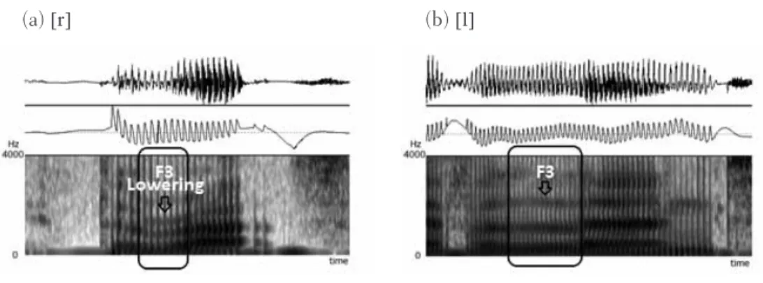
慶應義塾 外国語教育研究 第13号. they have clear formant frequencies. This provides them with vowel-like features, making these sounds acoustically distinct from other consonants. The sonority of these sounds is thus higher than other consonants, including plosives, fricative and affricates. Espy-Wilson (1992) noted these characteristics, and analyzed all four English approximants in terms of a decrease in energy at low frequencies, abrupt amplitude change, mid-frequency energy and the first four formants. F3 is recognized as one of the primary cues used to distinguish between  and  of all measurements. The decrease of F3 is a characteristic feature of , and the lowering of F3 in  has been measured in previous studies (Flege, Takagi et al., 1995; Iverson et al., 2001; Saito & Lyster, 2011). Flege, Takagi et al. (1995) highlighted the importance of lowering F3 for English , noting that a higher F3 value led to more perceived foreign accentedness. Figure 1.1 depicts F3 of  in rats and  in learn. The boxed portion in each spectrogram corresponds to the whole  and . The horizontal line immediately below the arrow is F3, measured in hertz (Hz). (a) . (b) . Figure 1.1. The spectrogram of  and : (a) ; and (b) . A relatively wider range of F3 values have been reported for English , which reflects a different degree of r-coloring. Some initial  was produced as low as 1240 Hz when articulated with a strongly curled tongue; in contrast, because of the lesser degree of r-coloring, F3 in the intervocalic  is lowered only to a smaller extent (Ladefoged, 2003). Ladefoged (2003) described the intervocalic  in berry as having the F3 value of 2100 Hz. Saito and Lyster (2011) maintained that the degree of F3 lowering affected native speaker judgment, reporting that  tokens with F3 values ranging from 2200 Hz to 2300 Hz were judged as good examples of English  of all tokens produced by Japanese learners of English.. 24.

Difficulty levels of English  and  for Japanese learners: An acoustic analysis. In contrast, as evident in a comparison with F3 of the sounds preceding and following  in Figure 1.1, F3 of  has no abrupt change. Flege, Takagi et al. (1995) found that the average F3 value of  produced by native speakers of American English was 2854 Hz. Saito and Lyster also noted that authentic  would be produced with F3 of 2800 Hz. Another acoustic cue of  to be noted is the presence of anti-formants (Kent & Read, 2002). The spectrogram of  in Figure 1.1, surrounded by vowels, shows that formants of  are also generally weaker than those of the adjacent vowels. Because  is articulated with. the tip of the tongue on the alveolar ridge, the air flow goes out through the side(s) of the oral cavity. This blockage causes the energy to radiate, which is reflected as anti-formants on the spectrogram, as with nasals. 1.4 Research question and hypotheses. This study aimed to examine the learning of  and  with a specific focus on production and to identify the difficulty level of these approximants by defining  and  as easy, learnable or difficult items for Japanese learners of English. To address this research question, hypotheses were formed as follows. It was hypothesized that  and  would be learnable and difficult, respectively. Both approximants do not have any exact counterpart in the Japanese phonological inventory as noted in Section 1.1, which suggests that Japanese learners have to learn both phones from scratch. Previous research shows that training (Saito & Lyster, 2001) and exposure or age (Slawinkski, 1999) would be key factors in promoting learning, and therefore, these findings imply no strong ground for hypothesizing that these approximants would be easy items. Additionally, some researchers claim that the degree of difficulty varies between  and  as far as production is concerned:  is more likely to be learned (Aoyama et al., 2004; Hazan et al., 2005). Although others argue that both approximants could be learned (Flege, Takagi, & Mann, 1995; Slawinski, 1999), it is not a major argument that  is easier than  for Japanese learners to learn to produce. Thus,  was predicted to be learnable and  to be difficult. 2. Methods 2.1 Participants. Ninety-one speakers participated in this study: 72 were Japanese learners of English ( JL), 12 were native speakers of British English (BN) and 7 were native speakers of American. 25.

慶應義塾 外国語教育研究 第13号. English (AN). The JL participants were third-year students at boys high school well reputed for its high academic level. They had diverse academic backgrounds, but none of them had the experience of living in an English-speaking country. The JL’s performance data were compared against those of BN/AN obtained from publicly available databases, the UCL Speaker Database (Markham & Hazan, 2002) and the Audio Archive (Merfert, 1997). The data of these speakers with two different accents were used because both are the most common accents of English taught in the classroom in Japan and spoken around the world. It is known that gender affects the absolute values of formant frequencies, and thus, this study only collected data from male speakers. 2.2 Materials. Phonetically-balanced passages, The Story of Arthur the Rat and Arthur the Rat, were used. Data for the BN and JL participants were collected using the former passage and those for the AN participants, using the latter. These passages were slightly different in some words used, but they follow exactly the same story line. Target words were selected from these passages. Voiced approximants,  and , occurred either at the word-initial position or the word-medial position as follows. The number within the square brackets in the list presents the number of repetitions, when provided: BN/JL data : rat [5], rainy, room, roof [2], right, rode, carry and hurry : learn, looked, lived, last, later, lying, Helen and Nelly AN data : rat [6], rainy, room, roof, right, rode, carry and hurry : like, look, loft, little, long, line, Helen and Nelly 2.3 Recording and procedure. All recordings of the JL participants were made using a digital recorder, Roland-09, and a condenser microphone, SONY ECM-MS957. Their data were recorded at a sampling rate of 44.1 kHz, 16 bit. The recording level was first checked and adjusted to each speaker. The material, printed on one side of A4 paper, was distributed to each participant between 3 days and 30 minutes prior to the recording. A summary of the story was presented in. 26.

Difficulty levels of English  and  for Japanese learners: An acoustic analysis. Japanese on the other side of the paper, with the intention of helping them to grasp the gist of the story. Although the participants were allowed to look up the pronunciation of unfamiliar words in a dictionary before the recording session, no instructions were given by the experimenter as to phonetic and phonological features. 2.4 Acoustic analyses. Based on the finding of Saito and Lyster (2011) that only F3 values predicted whether the native listeners would perceive a produced sound as , F3 was acoustically analyzed in this experiment. F3 was measured for  and , after the spectrogram and formant track were specified on Praat (Boersma & Weenink, 2011, 2015). Because the low F3 value characterizes  as described in Section 1.3, the lowest F3 values at the beginning of the upward slope and. the steady-state F3 value were measured for each token. The values were obtained in Hz. One thing that should be considered when analyzing the speech sample collected from non-native speakers is that the F3 values cannot be measured when another sound is substituted for the target  and . There were two cases of this; one was the substitution of a flap-like sound and the other was that of a vowel-like sound. The flap-like pronunciation is evident from the presence of a hold phrase in most cases. When the presence of the hold phrase could be confused with the presence of anti-formant for , a durational cue was applied to judge whether the token was  or a flap-like sound, referring to the duration of a flap obtained by Rimac and Smith (1984). Both durations and F3 values were therefore recorded with the candidates for the flap-like tokens that had an unclear hold phrase. The articulation rate, calculated using the script (de Jong & Wempe, 2009) on Praat (Boersma & Weenink, 2011, 2015), was also obtained so as to take into account the difference in the speaking rate between the BN/AN participants and the JL participants. The other type of substitution, vowel-like pronunciation, was due to an incomplete articulation of . The tokens were classified into this type of error, when characteristics of anti-formant were not visually evident in the spectrogram and waveform. 2.5 Variables for  and . Two variables were applied to the statistical tests on the production of  and : score for the  and score for the  tokens, which corresponded to the number of tokens produced as the intended sound as in Table 2.1. These variables were obtained by judging every target token as ,  or other sounds with reference to the BN/AN data, and counting the number. 27.

慶應義塾 外国語教育研究 第13号. of tokens identified as intended.. Table 2.1. Variables for the Analysis of  and  No. of variables. Level of measurement. Scale. Score for the  tokens. 1. Interval. 0-8. Score for the  tokens. 1. Interval. 0-8. Variable. After the F3 values were measured, they were converted from Hz to mel using Equation 1 (Fant, 1968): Mel = 1000/ log 210 x log(1+F/1000). (1). where F represents the frequency value. The thresholds of the F3 mel value to distinguish between  and  and that of the durational value to separate  from a flap-like sound were then set based on the data of BN/AN participants. As for the F3 threshold to classify the tokens into  or , all tokens of initial  and  obtained from the BN/AN participants were ranked according to F3, and the F3 mel values whose z-scores fell at 2 SD and -2 SD were defined as the thresholds for  and , respectively. The durational threshold for a flap-like sound, on the other hand, was set using the average duration of American flaps for adult speakers, reported by Rimac and Smith (1984), 33 ms, as a reference. Non-native speakers are likely to speak more slowly than native speakers (Munro & Derwing, 1995); therefore, a modified threshold for the JL participants was calculated by multiplying 33 ms by the ratio of the average articulation rate of the JL participants to that of the BN/AN participants. Every item was scored in terms of whether they were produced as intended or not, with reference to the threshold values above. First, by comparing the duration of the candidates for the flap-like tokens against the threshold of the durational value for a flap-like sound, tokens longer than the threshold were considered not to be flap-like. These tokens were submitted to the subsequent scoring process to judge whether or not the tokens were  or . The  tokens with F3 lower than threshold F3 value for  and the  tokens with F3 higher than the threshold F3 value for  were judged as intended. The two variables were obtained on a. 28.

Difficulty levels of English  and  for Japanese learners: An acoustic analysis. scale of 0 to 8 by adding the scores for the eight items of  and  each. The target word rat was repeated in the passage five times for the BN and JL data and six times for the AN data, and roof was repeated twice for BN and JL data. These words were scored as intended when more than one token was judged as intended for rat and when at least one token was judged as intended for roof. 2.6 Statistical analyses. Three statistical analyses were performed using the variables above: a cluster analysis, a multivariate analysis of variance (MANOVA) and a discriminant analysis. The first statistical test, a cluster analysis, was carried out to group the participants into clusters, based on similarities in the input variables. This analysis was conducted using the entire sample, including the BN/AN participants, which made it possible to form the groups of JL participants depending on similarities in their performances. The cutoff point was selected on two criteria. One is that at least one of the clusters consisted of as many BN/AN participants as possible, called a BN/AN cluster. This is based on the theoretical hypothesis that the BN/ AN participants would be grouped together. The other was that the JL participants formed four clusters at most, called as JL clusters, considering the balance of the sample size of each cluster for the subsequent analyses. The second statistical test, a MANOVA, was carried out using the clusters generated by this analysis as the between-subjects independent variables. It revealed whether there was a statistical difference among the clusters or not. The third statistical test, a discriminant analysis, was performed to identify clusters that differed in the variables at a statistically significant level. This judgment was based on the distance displayed in the canonical discriminant function plots and the location with reference to the group centroids indicated by positive and negative signs. A discriminant analysis additionally showed which variables discriminated them and to what degree these variables contributed to the discrimination. This was judged based on the structural matrix of the correlations between the variables and each of the discriminant functions. There is no decisive standard in the interpretation of the correlations, but those higher than .33 were interpreted to suggest variables contributing to the discrimination, following the convention provided by Tabachnick and Fidell (2007). 2.7 Criteria of learning. In order to define the difficulty level of  and  as easy, learnable or difficult, the results. 29.

慶應義塾 外国語教育研究 第13号. were discussed by comparing the BN/AN cluster(s) with the JL clusters. The definition was then given against the following criteria. The first criterion was whether the target item discriminated between the BN/AN cluster(s) and the JL clusters. The items that did not discriminate between the JL clusters and the BN/AN cluster(s) were interpreted as easy for Japanese learners of English. The second criterion was how many JL participants were discriminated from the BN/AN cluster(s) when the target items differentiated between the JL clusters and the BN/AN cluster(s). The items that discriminated more than half the JL participants from the BN/AN cluster(s) were defined as difficult items. The items that discriminated some JL participants from the BN/AN cluster(s), but not more than half the JL participants, were defined as learnable items. 3. Results. Before presenting the results of the score for the  tokens and the score for the  tokens, the threshold value of duration for a flap-like sound and the threshold values of F3 will be reported. As described in Sections 2.4 and 2.5, the threshold value of duration was computed to judge some  tokens as  or a flap-like sound. The articulation rate of the BN and AN participants was 4.44 syllables per second and that of the JL participants was 3.43 syllables per second on average, and the threshold was thus defined as 43 ms for the JL participants by multiplying 33 ms (Rimac & Smith, 1984) by 1.29. The 33 ms threshold of duration was applied to the BN/AN participants, and as a result of this threshold, six tokens produced by BN/AN participants were judged as a flap-like sound. The tokens defined as either  or  were then submitted to the scoring procedure to determine whether  and  were produced as intended using the threshold values of F3 for  and . The results of the BN/AN data showed that the F3 value of initial  at 2 SD and. that of initial  at -2 SD were 1665 mel Hz and 1671 mel Hz, respectively, and these values were set as the threshold value of F3 for each approximant. Three  tokens out of the 113 and two  tokens out of the 111 that the BN/AN participants produced were identified as unintended when these thresholds were applied. Table 3.1 and Figure 3.1 present the descriptive statistics of the variables for the BN, AN and JL groups. Figure 3.1(a and b) illustrates these variables, the average number of the  and  correct tokens out of eight and the average number of tokens for each error type,. respectively. In Figure 3.1(a), the items are indicated on the x-axis and the score for the  and  tokens on the y-axis. In Figure 3.1(b), the error types and the average number of errors. 30.

Difficulty levels of English  and  for Japanese learners: An acoustic analysis. are shown on the x-axis and y-axis, respectively. The errors were broadly categorized into three types, as displayed in the figure: the substitution of  for  and vice versa, that of a flap-like sound for  and  and that of a vowel-like sound for  and .. Table 3.1. Descriptive Statistics of  and  for BN, AN and JL Groups AN (n = 7). BN (n = 12). JL (n = 72). M. SD. Max. Min. M. SD. Max. Min. M. SD. Max. Min. . 7.83. 0.39. 8.00. 7.00. 7.57. 0.79. 8.00. 6.00. 2.86. 2.62. 8.00. 0.00. . 7.42. 0.67. 8.00. 6.00. 7.29. 0.76. 8.00. 6.00. 2.69. 2.34. 8.00. 0.00. Note. For  and , the highest possible value is 8, corresponding to the number of items.. (b) Number of errors. 8. 8. 7. 7. 6 5 4. BN. 3. AN. 2. JL. 1 0. r. l. Voiced Approximant. Average Number of Errors. Score of the Target Tokens. (a) Scores for the  and  tokens. 6 5 4. BN. 3. AN. 2. JL. 1 0. r>l. r > flap. r > vowel. l>r. l > tap. l > vowel. Error Type. Figure 3.1. Score for the  and  tokens and average number of errors for BN, AN and JL groups: (a) the score for the  and  tokens; and (b) the number of errors for six error categories. r>l = substitution of  for ; r>flap = substitution of a flap-like sound for ; r>vowel = substitution of a vowel-like sound for ; l>r = substitution of  for ; l>flap = substitution of a flap-like sound for ; l>vowel = substitution of a vowel-like sound for .. The BN and AN groups and the JL group primarily differed in the number of correct tokens as in Table 3.1. The JL group achieved lower scores for both  and  (M = 2.86, SD = 2.62 for ; M = 2.69, SD = 2.34 for ) than the BN group (M = 7.83, SD = 0.39 for ; M = 7.42,. SD = 0.67 for ) and the AN group (M = 7.57, SD = 0.79 for ; M = 7.29, SD = 0.76 for. 31.

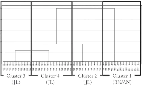
慶應義塾 外国語教育研究 第13号. ). Figure 3.1(a) displays no substantial difference in the scores between  and  for each. group, and also shows how low the scores of the JL group were, compared to those of the BN/AN groups. Figure 3.1(b), furthermore, reveals that the low score of the JL groups were attributed to frequent substitutions of both  and  for a flap-like sound. Substitutions of  for  and vice versa came next. A cluster analysis was carried out to profile the JL participants, using the z-scores of the scores for the  and  tokens calculated based on the mean and standard deviation of the entire sample. Figure 3.2 shows the dendrogram output by the analysis.. Cluster 3 ( JL). Cluster 4 (JL). Cluster 2 ( JL). Cluster 1 (BN/AN). Figure 3.2. Dendrogram for  and  All participants were separated into four clusters at the earliest stage of the clustering process. The four clusters were thus selected for the statistical analyses that followed. Cluster 1 consisted of 12 BN participants, 7 AN participants and 6 JL participants. This cluster was considered to represent native speakers, and termed as a BN/AN cluster (Figure 3.2). Clusters 2, 3 and 4 were comprised of 20 JL participants, 19 JL participants and 27 JL participants, respectively, each of which was termed as a JL cluster (Figure 3.2). Table 3.2 shows the descriptive statistics for the four clusters formed by the cluster analysis, where the valid F3 values averaged across participants were also presented. Some participants whose tokens were judged as neither  nor  failed to provide any valid F3 values; therefore, the number of participants from whom the F3 values were measured is also. 32.

Difficulty levels of English  and  for Japanese learners: An acoustic analysis. given in the table. Figure 3.3(a and b) visually presents the scores for the  and  tokens, and the average number of errors for each error type, respectively. The results are summarized in Figure 3.3(a and b) in the same style as Figure 3.1(a and b).. Table 3.2. Descriptive Statistics of  and  for Four Clusters. Valid F3 n. Cluster 1 (n = 25). Cluster 2 (n = 20). Cluster 3 (n = 19). Cluster 4 (n = 27). 25  / 25 . 20  / 18 . 13  / 19 . 14  / 19 . M. M. M. M. SD. SD. SD. SD. . 7.40. 1.15. 5.75. 1.41. 1.21. 1.03. 1.11. 1.22. . 7.28. 0.74. 1.55. 1.23. 4.95. 1.22. 1.00. 0.78. F3 Hz . 1735.33. 156.60. 1819.72. 102.23. 1789.36. 161.11. 1861.69. 156.89. F3 Hz . 2546.50. 131.71. 2562.12. 176.40. 2497.90. 140.04. 2565.37. 115.93. F3 mel . 1489.06. 69.40. 1491.40. 52.81. 1460.20. 81.78. 1487.68. 142.50. F3 mel . 1824.57. 52.31. 1830.76. 70.51. 1784.35. 56.42. 1833.13. 46.98. Note. The number given on the third row shows the number of participants who provided a valid F3 value of  and . For  and , the highest possible value is 8, corresponding to the number of tokens.. The four clusters had different patterns of performance for the production of  and , as clearly shown in Table 3.2 and Figure 3.3(a). The target tokens that the participants in Cluster 1, the BN/AN cluster, produced were most frequently judged as intended for both  and  (M = 7.40, SD = 1.15 for ; M = 7.28, SD = 0.74 for ). In contrast, Cluster 2 obtained a higher score for  than  (M = 5.75, SD =1.41 for ; M = 1.55, SD =1.23 for ), Cluster 3 achieved a higher score for  than  (M = 1.21, SD =1.03 for ; M = 4.95, SD = 1.22 for ) and Cluster 4 performed poorly for both  and  (M = 1.11, SD =1.22 for ; M = 1.00,. SD = 0.78 for ). These patterns are reflected in the pattern of errors that the participants in the JL clusters made. As can be seen in Figure 3.3(b), Cluster 2, which performed better in , substituted  for  most frequently, Cluster 3, which performed better in , tended to. substitute  for  or a flap-like sound, and Cluster 4, which performed most poorly in both  and , substituted a flap-like sound for  and  more often than the other clusters.. 33.

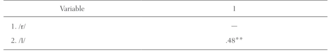
慶應義塾 外国語教育研究 第13号. (b) Number of errors. 8. 8. 7. 7. 6 5. Cluster 1. 4. Cluster 2. 3. Cluster 3. 2. Cluster 4. 1 0. r. l. Average Number of Errors. Score of the Target Tokens. (a) Scores for the  and  tokens. 6 5. Cluster 1. 4. Cluster 2. 3. Cluster 3. 2. Cluster 4. 1 0. r>l. r > flap r > vowel. Voiced Approximant. l>r. l > flap l > vowel. Error Type. Figure 3.3. Score for the  and  tokens and average number of errors for four clusters: (a) the score for the  and  tokens; and (b) the number of errors for six error categories. r>l = substitution of  for ; r>flap = substitution of a flap-like sound for ; r>vowel = substitution of a vowel-like sound for ; l>r = substitution of  for ; l>flap = substitution of a flap-like sound for ; l>vowel = substitution of a vowel-like sound for .. A one-way MANOVA was conducted with the scores for the  and  tokens as dependent variables, and the four clusters as the independent variables, in order to determine whether these visually detected differences were significant or not. Table 3.3 shows that two variables, the score for  the tokens and that for the  tokens, were moderately correlated. This suggests that a MANOVA was estimated to work well with these variables, as in Tabachnick and Fidell (2007), who states that the MANOVA does not perform well when the variables have an extremely high or low correlation.. Table 3.3. Correlation between the Variables for  and  Variable. 1. 1. . －. 2.. .48**. ** p < .01.. 34.

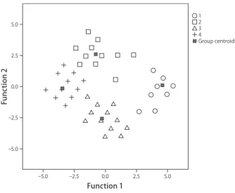
Difficulty levels of English  and  for Japanese learners: An acoustic analysis. The sample size of the largest cluster was less than 1.5 times as large as that of the smallest cluster, so that the á level was set at .05 (Stevens, 2007). Pillai’s trace yielded a significant difference among the clusters, F(6, 174) = 140.91, p < .001,. 2 p. = .83.. A post-hoc discriminant analysis was performed to identify the differences among the clusters, which was found by the MANOVA. Two discriminant functions were found to discriminate between the clusters. The first function accounted for 76.7% of the variance, canonical R2 = .91, and the second function accounted for 23.3% of the variance, canonical. R2 = .75. When combined, these functions significantly differentiated the clusters from each other with the Wilk’s lambda value of .02, ÷2(6) = 328.64, p < .001. After removing the first function, the second function was able to discriminate between the clusters at a significant level with the Wilk’s lambda value of .25, ÷2(2) = 120.70, p < .001. These results mean that the differences among the clusters can be explained by these two functions with the first function accounting more for the differences. The group centroids in Table 3.4 and the discriminant plot in Figure 3.4 show that the four clusters were well discriminated by the functions. The first function distinguished Clusters 2, 3 and 4 from Cluster 1. Cluster 1 and Cluster 4 were separated maximally. The second function differentiated between the JL clusters, where Cluster 2 and Cluster 3 were discriminated most.. Table 3.4. Group Centroids for  and  Function Cluster. 1. 2. 1. 4.58. 0.09. 2. ⊖ 0.78. 2.58. 3. ⊖ 0.28. ⊖ 2.59. 4. ⊖ 3.47. ⊖ 0.17. 35.

慶應義塾 外国語教育研究 第13号. 1 2 3 4 Group centroids. 5.0. Function 2. 2.5. 0.0. 2.5. 5.0. 5.0. 2.5. 0.0. 2.5. 5.0. Function 1. Figure 3.4. Canonical discriminant function plot for  and .. Table 3.4 is a structural matrix to show the correlations between the variables and the two functions. The results revealed that the score for the  tokens loaded on the first function most highly (r = .81), and that of  also loaded on it (r = .62). As noted above, the first function discriminated Cluster 1 from the other clusters, especially between Cluster 1 and Cluster 4. Taken together, the results suggest that both the score for the  tokens and the score for the  tokens contributed to discriminating Clusters 2, 3 and 4 from Cluster 1, Cluster 4 from Cluster 1 in particular, as seen in Table 3.2 and Figure 3.3(a). The participants in Cluster 1 performed best for  and  of all clusters, obtaining the highest scores (M = 7.40,. SD = 1.15 for ; M = 7.28, SD = 0.74 for ), whereas those in Cluster 4 performed most poorly, achieving the lowest scores for both  and  (M = 1.11, SD =1.22 for ; M = 1.00,. SD = 0.78 for ). Cluster 2 also achieved the lower scores for both target approximants (M = 5.75, SD = 1.41 for ; M = 1.55, SD = 1.23 for ) than Cluster 1. This was true of Cluster 3 (M = 1.21, SD = 1.03 for ; M = 4.95, SD = 1.22 for ). Thus, none of the JL clusters failed to attain the level of the BN/AN clusters for the production of  and .. 36.

Difficulty levels of English  and  for Japanese learners: An acoustic analysis. Table 3.5. Structural Matrix for the Correlations between the Variables for  and  and the Two Discriminant Functions Function Variable. 1. 2. Score for the  tokens. .81. ⊖ .59. Score for the  tokens. .62. .79. Note. The variables with the absolute value of correlations with the corresponding functions of .33 and above were highlighted in bold.. The second function concerned the discrimination among the JL clusters, as noted earlier. According to the structural matrix in Table 3.5, this function was identified by both the score for the  tokens (r = .79) and the score for the  tokens (r= -.59). As in the values presented in Table 3.2, Cluster 3 gained the higher score for the  tokens (M = 4.95, SD = 1.22) than Cluster 2 (M = 1.55, SD = 1.23). In contrast, Cluster 2 obtained the higher score for the  tokens (M = 5.75, SD = 1.41) than Cluster 3 (M = 1.21, SD = 1.03). The participants. in Cluster 4 failed to achieve such higher scores than those in the other JL clusters for both approximants (M = 1.11, SD =1.22 for ; M = 1.00, SD = 0.78 for ) as in Table 3.2. Accordingly, these results demonstrated that the second function particularly highlighted the differences between Cluster 2 and Cluster 3. The average number of errors in Figure 3.3(b) also emphasized these differences among the JL clusters, as described above. Cluster 2, which showed better performance in , produced  even for the  tokens more often than Clusters 3 and 4. Cluster 3, obtaining the higher score for the  tokens, were likely to substitute  for  more frequently than Clusters 2 and 4. Cluster 4 performed more poorly in both  and  than Cluster 2 and Cluster 3, which would be reflected in the most frequent substitution for a Japanese consonant, a flap-like sound. 4. Discussion 4.1 Findings. This study measured F3 values produced by the JL participants and BN/AN participants to examine the difficulty level of learning two English approximants  and . The results showed that a majority of the JL participants produced both consonants less accurately than. 37.

慶應義塾 外国語教育研究 第13号. the BN/AN participants. At the same time, two patterns of learning were found for the JL participants: one is the pattern that  is learned faster than  and the other is the one that  is learned faster than . The results of the experiment and the definition of the difficulty. level will be discussed in more detail below. To judge the target tokens as intended  or , the threshold values of F3 were defined for  and , respectively, as follows: 1665 mel Hz and 1671 mel Hz. These thresholds of  and  are equal to 2177 Hz and 2185 Hz, respectively, when mel was converted back to Hz. The. threshold of  in this study was close to the F3 value of  in Saito and Lyster (2011), who reported the F3 value between 2200 Hz and 2300 Hz. This value defined as the threshold for  in the present study would therefore be reasonable. On the other hand, the threshold of . defined was lower than the value that Saito and Lyster reported as F3 value of , 2800 Hz. Iverson and Kuhl (1996) also showed the F3 values for  and , which helped discuss whether the thresholds of this study were reasonable or not. They investigated the perceptual similarity underlying ,  and  within the framework of the native language magnet model, and found that an F3 value of the best exemplar for  was 1473 Hz, and that for  was 3478 Hz for one group, and 3329 Hz for the other. Compared with these values, the. threshold values  and  in the present study seemed higher and lower, respectively. As Iverson and Kuhl noted, however, the best exemplars tended to be more extreme. The stimuli were created by synthesizing female speech, and were tokens that constituted a simple syllable structure, CV, in Iverson and Kuhl. In contrast, the F3 values that this study set were not F3 values for good exemplars or averages, but thresholds. The values were defined based on the speech sample collected from male speakers, and a passage was used to collect the data. In addition, the phonetic boundary of F3 between  and , found by Iverson and Kuhl, was somewhere between 2067 Hz and 2523 Hz. The thresholds of this study fell within this range. Taken together, the thresholds of F3 defined in the present study would be acceptable. The cluster analysis was carried out using the variables obtained based on these yardsticks, and it generated one BN/AN cluster, consisting of 25 participants. All BN/AN participants were classified into this cluster. The fact that only six JL participants were grouped into the same cluster as the BN/AN participants suggests the overall difficulty of learning  and . The cluster analysis also formed three JL clusters, each of which comprised of 20 JL participants, 19 JL participants and 27 JL participants. All these clusters were discriminated from the BN/AN cluster in production of both  and . The results suggest that  and  were difficult items for the JL participants to learn to produce according to the criteria. 38.

Difficulty levels of English  and  for Japanese learners: An acoustic analysis. described in Section 2.7 because more than half the JL participants were differentiated from the BN/AN cluster. At the same time, it was found that there was a difference in the performances of both  and  among the JL participants, although none of the JL clusters reached the level of BN/ AN cluster. This points to some potential for learning by Japanese learners of English. The major difference was that the JL cluster of 20 participants performed better in producing , that the JL cluster of 19 participants performed better in  and that the JL cluster of. 27 participants performed poorly on both  and . This pattern was further supported by the results of the pattern of the errors that they made. The JL cluster of 20 participants produced  even for the  tokens, and  was thus an easier item than  for them to learn. In contrast, the JL cluster of 19 participants tended to substitute  for the  tokens more often, which suggests that  was an easier item than  for them to learn, unlike the JL cluster of 20 participants. The cluster of 27 JL participants were most likely to replace both  and  tokens with a flap-like sound of all clusters. This indicates that they did not have any preference for learning  or , but rather had been learning neither  nor . The statistical tests including a MANOVA and a discriminant analysis confirmed these. results that some of the JL participants had been learning  or , while the others had not. However, evidence of learning these approximants was only found in less than half of the JL participants. Accordingly, both target approximants were defined as difficult items. 4.2 Definition of the difficulty level. It was hypothesized that  and  would be learnable and difficult for Japanese learners of English, respectively. According to the results, more than half of the JL participants significantly differed from the BN/AN participants in production of both target approximants, and fewer than half of the JL participants improved their articulation of  and . Twentyseven JL participants, nearly half the JL participants, even performed poorly for both  and , and showed a high frequency of substitution of a flap-like sound for  and . Both approximants were thus identified as difficult items for Japanese learners of English to learn to produce, which rejected the hypothesis of  and upheld that of . The present research formed the hypothesis for  based on the findings of Aoyama et al. (2004) and Hazan et al. (2005) that  could be learned faster than . One of the possible reasons that this study failed to support this would be related to the proficiency level of the participants. Previous studies have found the difficulty for less experienced learners to attain. 39.

慶應義塾 外国語教育研究 第13号. the level of native speakers in production of  and  (Flege, Takagi et al., 1995; Goto, 1971), and have suggested a different status of  and  in the L2 phonological space of Japanese learners of English. Considering that the participants in this study were less experienced learners, who had no experience of living in an English-speaking country, the findings here were consistent with these past studies. Yamada (1995) pointed out that the experience of living in the U.S. could affect the perception of these approximants. Saito and Lyster (2011) reported that with training, Japanese learners of English could improve the production of . It was also found that there were  preference and  preference for learning, which was unexpected. The participants in one JL cluster showed that they were going through the learning process of , while those in another JL cluster were learning . This gives an indication that there are individual differences in the way of learning. It should be emphasized that some JL participants were learning  faster than , in particular. This is against the prediction of one of the learning models for production, the Speech Learning Model (SLM; Flege, 1987, 1995), which proposes that the newer L2 phones are easier for learners to learn while the more similar L2 phones to an L1 phone are more difficult. Guion et al. (2000) claimed that the difference between English  and Japanese  would be more salient than that between English  and Japanese , although no Japanese sound was perceptually similar to  and . From the articulatory perspective,  could also be assumed to be newer than . The major phonetic features of articulating English , such as retracted tongue or lip rounding, are not prominently used in Japanese. On the other hand, English  and Japanese  differ in that the former is continuant and the latter is not, but both require the tip of tongue as an active articulator and the alveolar ridge, or around this region, as a passive articulator. Thus, the newness is higher for . When the SLM is applied here, the higher degree of salience of  can facilitate Japanese learners learning this approximant. However, this did not hold true of this study that demonstrated that some learners were learning  faster. Thus, the findings in this study suggest the need to test one of the most influential learning models, the SLM, although it should be taken into account that the participants in the present study were not so experienced as the SLM requires learners to be experienced for its prediction. 5. Conclusion. The present study aimed to define  and , notoriously difficult for Japanese learners of English to learn to produce, as easy, learnable or difficult items. The results showed that. 40.

Difficulty levels of English  and  for Japanese learners: An acoustic analysis. both approximants were difficult. However, it was also found that there was an individual preference about which approximant was learned faster. Some Japanese learners of English were learning  faster than  whereas others were learning  faster than . Further studies will be required to explore from what these individual differences arise, and how positively the preference for learning  or  will affect the learning of both approximants.. References Aoyama, K., Flege, J. E., Guion, S. G., Akahane-Yamada, R., & Yamada, T. (2004). Perceived phonetic dissimilarity and L2 speech learning: The case of Japanese  and English  and . Journal of. Phonetics, 32(2), 233-250. Boersma, P., & Weenink, D. (2010). Praat: doing phonetics by computer (Version 5.2) [Computer program]. Retrieved from http://www.praat.org/ Boersma, P., & Weenink, D. (2015). Praat: doing phonetics by computer (Version 6.0.05) [Computer program]. Retrieved from http://www.praat.org/ Espy-Wilson, C. Y. (1992). Acoustic measures for linguistic features distinguishing the semivowels  in American English. Journal of the Acoustical Society of America, 92(2), 736-757.. Fant, G. (1968). Analysis and synthesis of speech processes. In B. Malmberg (Ed.), Manual of phonetics (pp. 173-177). Amsterdam, the Netherlands: North-Holland. Flege, J. E. (1987). The production of “new” and “similar” phones in a foreign language: Evidence for the effect of equivalent classification. Journal of Phonetics, 15(1), 47-65. Flege, J. E. (1995). Second language speech learning: Theory, findings, and problems. In W. Strange (Ed.), Speech perception and linguistic experience: Issues in cross-language research (pp. 233-277). Timonium, MD: York Press. Flege, J. E., Takagi, N., & Mann, V. (1995). Japanese adults can learn to produce English  and  accurately. Language and Speech, 38(1), 25-55. Goto, H. (1971). Auditory perception by normal Japanese adults of the sounds “L” and “R.”. Neuropsychologia, 9, 317-323. Guion, S. G., Flege, J. E., Akahane-Yamada, R., & Pruitt, J. C. (2000). An investigation of current models of second language speech perception: The case of Japanese adults’ perception of English consonants. Journal of the Acoustical Society of America, 107(5), 2711-2724. Hallé, P. A., Best, C. T., & Levitt, A. (1999). Phonetic vs. phonological influences on French listeners’ perception of American English approximants. Journal of Phonetics, 27(3), 281-306. Hazan, V., Sennema, A., Iba, M., & Faulkner, A. (2005). Effect of audiovisual perceptual training on the perception and production of consonants by Japanese learners of English. Speech Communication,. 47, 360-378.. 41.

慶應義塾 外国語教育研究 第13号. Iverson, P., & Kuhl, P. K. (1996). Influence of phonetic identification and category goodness on American listeners perception of  and . Journal of the Acoustical Society of America, 99(2), 1130-1140. Iverson, P., Kuhl, P. K., Akahane-Yamada, R., Diesch, E., Tohkura, Y., Kettermann, A., & Siebert, C. (2001). A perceptual interference account of acquisition difficulties for non-native phonemes. Speech,. Hearing and Language: Work in progress, 13, 106-118. de Jong, N. H., & Wempe, T. (2009). Praat script to detect syllable nuclei and measure speech rate automatically. Behavior Research Methods, 41(2), 385-390. Kent, R. D., & Read, C. (2002). Acoustic analysis of speech (2nd ed.). Clifton Park, NY: Delmar. Ladefoged, P. (2003). Phonetic data analysis: An introduction to field work and instrumental techniques. Malden, MA: Blackwell. Markham, D., & Hazan, V. (2002). The UCL speaker database. Speech, Hearing and Language: Work in. Progress, 14, 1-17. Merfert, I. (1997). The alt.usage.english Audio Archive. Retrieved from http://alt-usage-english.org/index. shtml Munro, M. J., & Derwing, T. M. (1995). Processing time, accent, and comprehensibility in the perception of native and foreign-accented speech. Language and Speech, 38, 289-306. Rimac, R., & Smith, B. L. (1984). Acoustic characteristics of flap productions by American Englishspeaking children and adults: Implications concerning the development of speech motor control.. Journal of Phonetics, 12(4), 387-396. Saito, K., & Lyster, R. (2011). Effects of form-focused instruction and corrective feedback on L2 pronunciation development of  by Japanese learners of English. Language Learning, 62(2), 595633. Slawinski, E. (1999). Acquisition of /r-l/ phonemic contrast by Japanese children and adults.. Psycholinguistics on the Threshold of the Year 2000, 583-590. Stevens, J. P. (2007). Intermediate statistics: A modern approach (3rd ed.). New York, NY. Routledge. Tabachnick, B. G., & Fidell, L. S. (2007). Using multivariate statistics (5th ed.). Boston, MA: Pearson Education. Yamada, R. (1995). Age and acquisition of second language speech sounds perception of American English  and  by native speakers of Japanese. In W. Strange (Ed.), Speech perception and. linguistic experience: Issues in cross-language research (pp. 305-320). Timonium, MD: York Press.. 42.