Jean-Antoine Seon, Brahim Tamadazte, and Nicolas Andreff
Abstract—Laser surgery requires accurate following of a path defined by the surgeon, while the velocity on this path is depen-dent on the laser–tissue interaction. Therefore, path following and velocity profile control must be decoupled. In this paper, nonholo-nomic control of the unicycle model is used to implement velocity-independent visual path following for laser surgery. The proposed controller was tested in simulation, as well as experimentally in sev-eral conditions of use: different initial velocities (step input, succes-sive step inputs, sinusoidal inputs), optimized/nonoptimized gains, time-varying path (simulating a patient breathing), and complex curves with curvatures. Thereby, experiments at 587 Hz (frames/s) show an average accuracy lower than 0.22 pixels (∼10µm) with a
standard deviation of 0.55 pixels (∼25µm) path following, and a
relative velocity distortion of less than10−6%.
Index Terms—Endoluminal interventions, intracorporal micro-robotics, laser surgery, nonholonomic control, surgical robot, vision-guided laser, visual servoing.
I. INTRODUCTION
L
ASER surgery consists of the use of a surgical laser (in-stead of a scalpel) to cut tissue in which the laser beam vaporizes the cells. A large variety of surgical areas practice laser surgery: ophthalmology, gynecology, otolaryngology, neu-rosurgery, and pediatric surgery [1]. This is especially trueManuscript received December 22, 2014; accepted January 30, 2015. Date of publication March 2, 2015; date of current version April 2, 2015. This paper was recommended for publication by Editor B. J. Nelson upon evalua-tion of the reviewers’ comments. Part of this work was presented at the 3rd Workshop on Visual Control of Mobile Robots (ViCoMor), IEEE/RSJ Interna-tional Conference on Intelligent Robots and Systems (IROS), 2014. This work was supported byµRALP, the EC FP7 ICT Collaborative Project no. 288663 (http://www.microralp.eu), and by ACTION, the French ANR Labex no. ANR-11-LABX-01-01 (http://www.labex-action.fr).
The authors are with the FEMTO-ST Institute, AS2M Department, Universit´e de Franche-Comt´e/CNRS/ENSMM/UTBM, 25000 Besanc¸n, France (e-mail: ja. [email protected]; [email protected]; Nicolas.Andreff@femto-st. fr).
This paper has supplementary downloadable material available at http://ieeexplore.ieee.org, provided by the author. The material consists of a video, viewable on—Windows systems: windows media player (version 11 or more) and VLC media player (version 1 or more) or Linux systems. The video file can be viewable in VLC media player (version 1 or more). The video (*.avi) presents the task, experimental set-up and also show how a developed C++ and OGRE Simulator illustrating the principle of the robotic laser phonosurgery. It shows also the operating of the developed approach in several conditions of works using a homemade experimental set-up. Since the work is about laser steering, especially for surgical applications, the video clearly demonstrates the validation of developed of a decoupling path following and velocity profile method at different experimental and simulation conditions. The experimental set-up includes a high speed camera, a 2 degrees of freedom steered mirror based on piezoelectric actuators, a fixed mirror, and a laser source. The obtained results illustrates that the following accuracy in about 0.22 pixels (∼10µm) with a very low velocity distorsion (7.5×10⁻⁸%). The size of the video is 6.68 MB.
Contact [email protected] for further questions about this work. Color versions of one or more of the figures in this paper are available online at http://ieeexplore.ieee.org.
Digital Object Identifier 10.1109/TRO.2015.2400660
when it comes to microsurgery, which requires an extreme precision [2].
For instance, vocal folds surgery is extremely demanding in terms of accuracy because of the specific tissue to be resected (thin, viscous, fragile, difficult healing, and lesions that can be less than 1 mm) and the necessity to preserve the patient’s voice [3], [4].
Currently, the most successful protocol for vocal folds surgery, widely used in hospitals, is certainly the suspension laryngoscopic technique, which consists of a straight–rigid laryngoscope, a stereomicroscope, a set of specific and minia-tures surgical instruments, a laser source, and a foot-pedal con-troller device to activate the laser [3]. In fact, the most popular microphonosurgery procedure uses the AcuBlade system [5], which allows good diagnostics and microsurgeries procedures. However, this system suffers from several drawbacks, especially in terms of accuracy (laser source placed outside the patient at 400 mm from the vocal folds) and ease of operation (teleopera-tion mode only). Consequently, the laser surgery performances are highly dependent on the individual surgeon dexterity and skills [6].
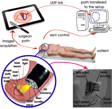
Generally, in the case of laser surgeries, the control consists of two tasks. The first one is to ensure the laser velocity com-patibility with laser–tissue interaction (longitudinal control), in order to avoid carbonization of the tissue, while achieving an ef-ficient incision or ablation. The second one (lateral control) is to ensure that the laser follows the desired geometric path drawn by the surgeon on the input device (e.g., a tablet in [7]) (see Fig. 1). These two tasks eventually define the trajectory (i.e., geometric path + velocity profile along the path) of the laser. However, it is not advisable to use standard trajectory tracking because the two tasks should be intuitively modifiable by the surgeon. In fact, the velocity of the laser displacements must be the same regardless of the shape, the size, or the curvature of the incision path. In addition, the norm of this velocity must be adapted, by the physician, in function of the tissue to be re-sected (thin, thick, fragile, etc.) or the laser source (CO2 laser,
Helium–neon laser, etc.). In this paper, we focus especially on the second task: laser path following using the visual feedback independently from the velocity profile.
Moreover, beyond laser surgery applications, efficient path following in which the velocity profile (easily tuned) is invari-ant to the path (nonparametrized curve) size, shape, curvature, sampling period, etc., can be an important issue for industrial applications that use laser scanning process. There are sev-eral works reported in the literature, especially in vision-based control supervision of welding process [8] or trajectory track-ing (with low curvature) ustrack-ing a robotic arm, which embeds the laser source [9]–[11]. In addition, regular and precise path following could find applications in 2-D/3-D laser
Fig. 1. Global view of the vocal folds surgery procedure.
Fig. 2. Block diagram for the unicycle kinematic model.
chining (e.g., microsystems fabrication) [14], as well as in free-contact micromanipulation techniques (e.g., laser trapping) [15]. Yet, as far as we could understand it, all those work use trajec-tory tracking instead of path following, making the longitudinal controller blind to variations in laser-matter interaction.
The first contribution of the paper is to consider, on purpose, laser path following as a nonholonomic problem, similar to unicycle path following. The second contribution of this paper is to implement path following at high frequency to satisfy the constraints of laser–tissue interaction.
In the remainder of this paper, Section II relates laser path fol-lowing in the image and unicycle path folfol-lowing on the ground. In Section III, a background on the existing path-following methods is given, while Section IV deals with the implemen-tation for laser path following technique. Section V presents simulation results, as well as experimental validation.
II. LASERPATHFOLLOWING IN THEIMAGEversus.UNICYCLE PATHFOLLOWING ON THEGROUND
Let us first show that laser path following in the image is very similar to unicycle path following on the ground (represented by the block diagram shown in Fig. 2)
1) in both cases, the direction and the amplitude of the ve-locity are served independently;
2) in the unicycle case, the velocity is generally expected to be such that the curvilinear velocity is constant, while in
Fig. 3. Block diagram for the laser steering kinematic model.
Fig. 4. Similarities between unicycle vehicle kinematic model (a) and a laser steering kinematic model (b).
the case of laser surgery, the velocity is expected to match a constant velocity on the tissue surface;
3) in both cases, the path following accuracy is expected to be independent from the velocity amplitude.
4) both laser spot and unicycle velocities should be smooth. With respect to these similarities, we thus chose to implement the unicycle model for the path following in the image. Indeed, imposing the unicycle nonholonomic constraint on the holo-nomic laser manipulator as shown in Fig. 3, which represents the laser steering kinematic model developed in this paper. This allows us to
1) ensure smoothness of the laser motion which is a key issue in laser surgery quality;
2) control the laser displacement with a uniform velocity along the path;
3) exploit efficient path following algorithms.
III. PATHFOLLOWING
A. State of the Art
Path following in mobile robotics has been widely studied in the literature for many years and has found several applica-tions in the industrial field (e.g., autonomous vehicle control [13], farming application [12]). Path following differs from tra-jectory following essentially by the fact that the notion oftime is removed in the first one. Indeed, in trajectory following the robot is controlled to be at a location at a given time, which is not the case in path following. Indeed, as shown by Brockett [16], mobile robots are not stable with continuous steady-state feed-back laws. The first alternative approach is to use discontinuous control laws [17] or piecewise continuous control law [18], but these methods do not explicitly address the issue of robustness to the occurrence of uncertainties. Thereafter, Hespanhaet al. [19] proposed to use a sliding mode-based controller, which has shown better behaviors. The second approach is to use con-tinuous non-steady-state feedback laws, such as Samson in the early 1990s [20]. Lyapunov methods are often used to design such type of control law [21], [22]. Indeed, it gives good results in terms of robustness and accuracy. It is also possible to use a chained system to design the controller with exact linearization as shown by Morin and Samson [23], [24]. In these studies, the path following speed profile is not known. Therefore, only the path and the distance between the robot and the curve are con-sidered. Therefore, the tangential vectors of the curve are used to set the velocity and the orientation of the robot.
B. Notations
For a better understanding of the different notations intro-duced in this paper, the reader may refer to Table I.
C. Kinematic Equations
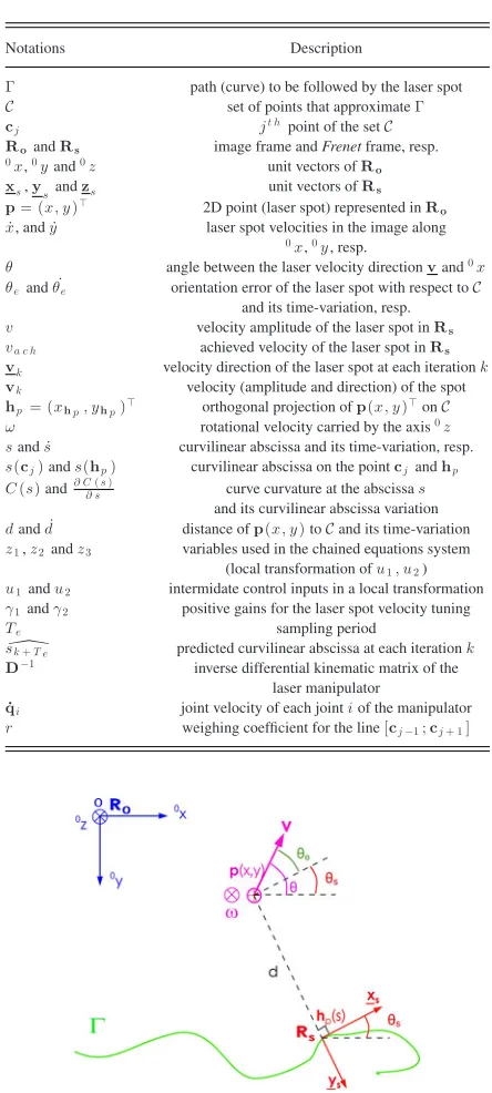
Let us consider the mobile robot (laser spot) represented by a 2-D point p= (x, y)⊤ in a fixed (reference) frameR
o (the
image frame). The kinematics of the unicycle are governed in the world frame by
˙
x= vcosθ (1)
˙
y = vsinθ (2)
˙
θ= ω (3)
where θ is the angle between laser velocity direction v and the 0xaxis of the world frame,v represents the translational velocity amplitude of the laser spot in Rs (v =vvk), hp(s) is the orthogonal projection of p = (x, y)⊤ on Γ, and ω its rotational velocity carried by the axis0z(see Fig. 5).
These equations can be generalized in theFrenetframeRs
attached to the path (see Fig. 5) as shown by Morin and Samson [23], [24]. Consequently, the kinematics become governed in
C set of points that approximateΓ
cj jt hpoint of the setC
RoandRs image frame andFrenetframe, resp.
0x,0yand0z unit vectors ofR
o
xs,ysandzs unit vectors ofRs
p= (x, y)⊤ 2D point (laser spot) represented inR
o
˙
x, andy˙ laser spot velocities in the image along 0x,0y, resp.
θ angle between the laser velocity directionvand0x
θeandθ˙e orientation error of the laser spot with respect toC
and its time-variation, resp.
v velocity amplitude of the laser spot inRs
va c h achieved velocity of the laser spot inRs
vk velocity direction of the laser spot at each iterationk
vk velocity (amplitude and direction) of the spot
hp= (xhp, yhp)⊤ orthogonal projection ofp(x, y)⊤onC
ω rotational velocity carried by the axis0z
sands˙ curvilinear abscissa and its time-variation, resp.
s(cj)ands(hp) curvilinear abscissa on the pointcjandhp
C(s)and∂ C∂ s(s) curve curvature at the abscissas
and its curvilinear abscissa variation
dandd˙ distance ofp(x, y)toCand its time-variation
z1,z2andz3 variables used in the chained equations system (local transformation ofu1, u2)
u1andu2 intermidate control inputs in a local transformation
γ1andγ2 positive gains for the laser spot velocity tuning
Te sampling period
sk+T e predicted curvilinear abscissa at each iterationk
D−1 inverse differential kinematic matrix of the laser manipulator
˙
qi joint velocity of each jointiof the manipulator
r weighing coefficient for the line[cj−1;cj+ 1]
Fig. 5. Representation of the different frames used in the design of the path-following method.
Rsby
˙
s= v
1−dC(s)cosθe (4) ˙
d= vsinθe (5)
˙
θe = ω−sC(s)˙ (6)
vand the tangential vector ofRsanddis the shortest distance
ofp= (x, y)⊤toΓ.
D. Control Law
To establish the controller, Samson [23] introduced a coordinates/variables transformation in the following man-ner: {s, d, θe, v, ω} ⇐⇒ {z1, z2, z3, u1, u2} defined in R2×
whereu1andu2are intermediate control inputs.
Thereby, ifz1=s, then (7) implies
As a consequence and using (9),u2is defined as
u2 = (−dC˙ (s)−d
∂C(s)
∂s s˙) tanθe
+ (1−dC(s))(1 + tan2θe)(ω−sC˙ (s)). (12)
Finally, to ensure that the distancedand the orientation er-rorθe are servoed to 0, the stable proportional state feedback solution [23] is
u2 =−u1γ1z2− |u1|γ2z3 (13)
whereγ1 andγ2 are positive gains andu1 = 0can be chosen
arbitrarily.
E. Stability Conditions
Therefore, the controller is asymptotically stable whenu1 =
˙
s is constant (positive or negative). However, the system is not controlled directly byu1 but byv. Therefore, a stability
condition on v is needed. It has been shown in [24] that the stability is ensured with
1) vmust be a bounded differentiable time-function, 2) vmust not tend to zero whenttends to infinity, 3) v˙must be bounded.
IV. IMPLEMENTATION
A. Laser Surgery Considerations
Up to now, the parameters of the curveΓare considered as perfectly known as in the case of the path planning for mobile robotics. Remind that in laser surgery, the controller receives the normalized and sampled coordinates of the path, while the sur-geon drawsΓ(using a tablet) as illustrated in Fig. 1. Therefore, the path used to control the laser displacements is an approxima-tion (yet very accurate) of the real curve drawn by the surgeon. As the curvatureC(s)needs to be computed for the control law, the parameterized path has to be at leastC2 (C(s)is the
time-derivation of the tangent vector). However, the fact that the path is a nonparameterized curve, then the curvature and the radius at each point are computed using three successive points. Obviously the quality of this approximation and the smoothness of the path depend on the number of points.
Consider that the pathΓis described by a set of pointsC= {ci,i= 1. . . n}with the relationc1 <c2 <· · ·<cn. Each ci is a quadruplet containing two Cartesian coordinates (x,y) and two curvilinear coordinates (curvatureC(s)and curvilinear abscissas).
In order to control the laser spot displacements with regards to the path drawn by the surgeon, the following methodology (Algorithm 1) has been developed, implemented, and validated in simulation and experimental setup.
Algorithm 1:Control loop for laser steering
v←laser speed
initialization←1
whilenot end of the pathdo
I←grab image() ifinitialization= 1then
( ˙x,y˙)←xs
∂ s ←curvature variations
(s, spr ev .iter., C(s), C(s)pr ev .iter.)
( ˙s,d˙)←kinematic equations(v, θe, d, C(s)) (u1, u2)←control law( ˙s, d,d, θ˙ e, C(s),∂ C∂ s(s))
ω←new rotational velocity
(u2,s, d,˙ d, θ˙ e, C(s),∂ C∂ s(s))
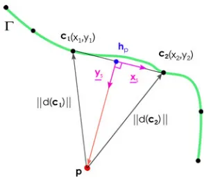
B. Computation of the Closest Point on the Path
searching through all the curve and be caught in ambiguities when, for instance, the path cross itself. In addition, usingcj andcj±1 allows us to compute the line projection ofpon the
approximated pathCwhich giveshp = (xhp, yhp)
which can be computed using
r= (xm in(cj,cj±1)−xm ax(cj,cj±1))(xm in(cj,cj±1)−xk)
ris also useful in case where the points ofC are not homo-geneously distributed. Indeed, ifr>1 then the projection of the laser spot will be outsideΓ(the two closest points are not the two points describing the segment on which the laser spot should be located).
C. Computation of the Laser State in the Frenet Frame
First, the curvilinear coordinates of the pointhpcan be easily computed. Thus, the curvilinear abscissas(hp)is computed as the addition of the curvilinear abscissa ofmin(cj,cj±1)and the
distance between this point andhp, and the curvatureC(s)in hp(i.e.,C(hp)) is computed as follows:
C(hp) = C(s(min(cj,cj±1)))(1−r)
+ C(s(max(cj,cj±1)))r. (18)
Moreover, the unit-vectorsxsandy
sdefining theFrenetframe Rsare determined using the line betweencj andcj±1as shown
in Fig. 6. Furthermore,dis recomputed using
d= (pk−hp)·ys (19)
where(pk −hp)is the normal vector alongysfrom the closest point to the laser spot position (see Fig. 6) and the dot product (·) allows knowing the exact sign of the laser spot position relative to the curveΓ. As theFrenetframeRsis constructed directly
on hp, it ensure that the two vectors ((pk −hp)andys) are always collinear.
Therefore, the orientation errorθeat each iterationkcan be updated by
wherevkis the current velocity direction of the laser spot in the R0frame.
Fig. 6. Estimation of the distancedat each iterationk.
D. Initialization
As shown in (20),vk is needed to compute the angle values at each iterationk. To do this, initialization values are fixed in order that the laser spot follows immediately the direction of the path. Thereby, the initial velocity of the laser spot is given by
v0=vxs. (21)
E. Constant Velocity Laser Steering
By knowing the laser spot state in theFrenetframeRs and
by inverting (12), it is possible to define the new expression ofω
From the latter, we derive the new expression of the laser spot velocity direction in the image by
vk+ 1 = vk +ω
where×defines the cross product andvk represents the current velocity direction of the laser spot.
Thereafter, it is necessary to convert these velocities to the joint velocities ˙qi (i∈[1,2]) through the inverse differential kinematic matrixDin v of the robot holding the laser as ˙qi = Din vvk+ 1.
V. VALIDATION
A. Experimental Setup
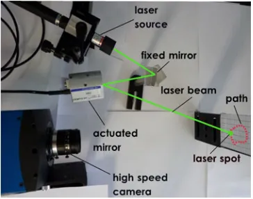
Fig. 7. Photography of the experimental setup.
Due to the low motion range of the PI mirror (i.e.,≡3◦), it is impossible to scan a region of interest of 20 mm×20 mm, which represent the average surface of vocal folds of an adult male (a little bit smaller for a female subject). It is for this reason that the target surface is positioned at a distance of 200 mm of the actuated mirror. However, we are working on the development of a large motion micromirror, which will able to gives laser beam rotations of 43◦in each dof.
Concerning the time-varying positionpof the laser spot in the image, it is tracked using ViSP library [25]. The tracking method is based on the computation of the gravity center (barycenter) of the laser spot in the image, i.e, a subpixel detection (in laser surgery, the laser spot has a size (diameter) of about 200µm).
B. Simulation Validation
The proposed method is first validated in simulation in order to verify the relevance of the proposed path following scheme and define optimally some initial parameters of the technique (suchv,γ1, andγ2) in different cases of use (shape and size of
the curve, velocity profile, sampling period, simulation of the tissue interaction, etc.).
1) Example of a Simulation: To illustrate the simulation re-sults, we opted for a nonparametric and arbitrary shape curve as shown in Fig. 8(a). In order to illustrate the relevance of the proposed approach, the initial parameters (gains) are tuned to get a laser velocityv=20 pixels/s,γ1=0.2, andγ2=0.8.
In this example, the initial position of the laser spot is placed with an initial orientation errorθe=0 rad and an initial distance
d=−15 pixels. The laser spot is deliberately placed away from the curve in order to test how the system will respond to large error. The simulation results are given in Fig. 8, where Fig. 8(a) shows the evolution of the laser spot positionprelatively to the reference curveΓ, and Fig. 8(b) and (c) illustrates the evolution of the distance errordand the orientation errorθe, respectively, versusnumber of iterationsk. It can be noted that once the laser spot joined the curveΓ,dandθeare maintained at 0.
To estimate the accuracy of the proposed method, we com-pute the RMS error and the standard deviation (STD) indand θe. It gives the following values: RMS(d) = 0.1466 pixels, STD(d)= 0.1253pixels, RMS(θe)= 0.2138rad, and STD(θe)= 0.2138 rad.
Fig. 8. Simulation results: (a) represents the path following achievement, (b) and (c) show the evolution ofθeandd, respectively.
Fig. 9. Study of the influence of the gainsγ1andγ2in the errors indandθe.
2) Gains Tuning: In order to determine the best couple of gains for the controller, several simulations are performed using the same curveΓ(see Fig. 8) with varyingγ1andγ2. Then, the
accuracy of each path following simulation is compared using four criteria: RMS of the error in distance along the pathdand its STD, and the RMS of the orientation errorθe and its STD (see Fig. 9). This curve alternates between areas of high and low curvature, but between different directions as well; therefore, it is a good template for estimating the best parameters.
The gains used for these simulations are included in the range [0.01,5]with a step of0.005of each gain. The results are shown in Fig. 9, where the closest values to 1 represent the best results. It can be highlighted that the error in distance along the path can be improved just by increasing the value ofγ1. This is directly
related to the (13), where γ1 controls the variable z2 which
representsd. In the same manner, increasingγ2will reduce the
Fig. 10. Various velocity profiles inputs during the path following process. (a) successive step inputs and (b) sinusoid inputs.
TABLE II
RMSANDSTDFORd(PIXELS)ANDθe(RAD)
vprofile RMS (d) STD (d) RMS (θe) STD (θe)
constant 0.0086 0.0080 0.0195 0.0195 sinusoidal inputs 0.0073 0.0065 0.0174 0.0174 steps inputs 0.0086 0.0078 0.0198 0.0198
both distance and orientation errors becauseγ2not only depends
onθebut can interfere withγ1, which may cause a disturbance
in the controller.
With these simulations, the computed optimal gains on the range [0.01,5] are located inγ1 = 5, γ2 = 0.71 considering
that bothθeandderrors have the same impact on the quality of the path following. This set of gains gives the following errors: RMS(d)= 0.0116pixels, STD(d)= 0.0106pixels, RMS(θe)= 0.0169rad, STD(θe)= 0.0169rad. However, even with nonop-timized parameters (example shown above), the proposed con-troller remains accurate, reliable, and stable.
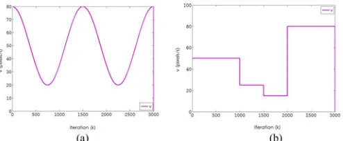
3) Impact ofvDuring the Path Following Achievement: As mentioned above, in laser surgery, the velocity of the laser spot in the tissue needs to be adapted with respect to the tissue surface, heat profile, depth of lesion, etc. Therefore, in order to illustrate that the developed controller can be used in such application, a simulation has been performed in an unknown shape path following with arbitrary change of the velocityvduring the path following process. To do that, two velocity profiles are used: the first is with a smooth variation (sinusoidal profile) during the process [see Fig 10(a)] and the second using a successive step inputs [see Fig. 10(b)]. The gains used for these simulations are optimized (γ1 = 5 and γ2 = 0.71) and the two velocity
profiles are compared with a path following at a constant speed of v=100 pixels/s. Through the results shown in Table II, it can be highlighted that the variation of the velocity during the path following process has no any impact on the quality of the following process. Indeed, the variation ofdandθe are in the same range with and without velocity variation.
4) Impact of Γ Variation During Path Following Process: Not being able to validate the controller on true tissues surface (especially on vocal cords), we simulated a curve (Γ(t)) whose size changed with a frequency close to that of a patient breathing. This experimentation is shown in Fig. 11, which rep-resents a captured image during the path following simulation in a variable curve (see multimedia Extension 1). This test
demon-Fig. 11. Image captured during the simulation with a path following with a time-varying curve.
Fig. 12. Image sequence captured during the experimental validation of the path following in the case of unknown shape curve. (a) represents a color image of a 3-D ham piece (similar in the texture and the aspect to the vocal folds tissues), and (b) to (f) illustrate the laser spot displacement following the reference path.
strates that despite the curve variation during the path following achievement, the accuracy remains more than satisfactory i.e., RMS(d)=0.0208 pixels, STD(d)=0.0204 pixels and RMS(θe) =0.2447 rad, STD(θe)=0.02445 rad.
C. Experimental Validation
The simulation tests have been reproduced on the experi-mental setup presented above. Therefore, the path chosen is the arbitrary shape curve used in the simulation section. The initial position of the laser spot is placed at a distanced=10 pixels with an initial orientation errorθe = 0. This is done again in order to evaluate how the system responds to important error (10 pixels=1000 times the RMS error). To do this, the initial parameters are fixed as follows:v=20,γ1=0.2, andγ2=0.8.
It can be underlined that the initial errors, as well as the initial parameters are chosen in a nonoptimal configuration (i.e., huge distance between the laser spot position and the curveΓ and nonoptimized gains) in order to evaluate the robustness of the controller.
er-Fig. 13. Evolution ofdandθefor the path following validation test shown
in Fig. 12.
Fig. 14. Velocity profile(v−va c h)
v and velocity progresss˙during the
valida-tion test shown in Fig. 12.
TABLE III
RMSANDSTDFORd(PIXELS)ANDθe(RAD)
N◦ RMS (d) STD (d) RMS (θ
e) STD(θe)
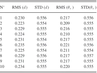
1 0.230 0.556 0.217 0.556 2 0.223 0.554 0.209 0.555 3 0.229 0.555 0.216 0.555 4 0.224 0.555 0.210 0.555 5 0.231 0.554 0.217 0.555 6 0.235 0.556 0.221 0.556 7 0.225 0.554 0.211 0.554 8 0.229 0.556 0.217 0.557 9 0.231 0.555 0.217 0.555 10 0.234 0.555 0.220 0.555 Each line represents the average of 3 individual tests.
ror distancedand Fig. 13(b) the orientation errorθeversusthe iterations number k(each iteration takes 1.702 milliseconds). In addition, it can be noticed that despite the oscillations ofθe, namely in low curvatures areas, this does not affect the quality of the path following i.e., the accuracy (given by the distance errord) remains high (≈0.22 pixels).
The velocity profile of this test is presented in Fig. 14(a), as well as the velocity of the laser displacement in Γ is shown in Fig. 14(b). It demonstrates that the velocity remains con-stant (with a relative velocity distortion(v−va c h)
v below 10
−6%)
between the achieved velocityvachand the desiredv.
D. Repeatability of the Path-Following Method
First, for a better assessment of the obtained results, the pre-vious test was reproduced 30 times by changing the initial po-sitions of the laser spot to the curveΓat each test. Thereby, the RMS errors indandθe, as well as the STD were computed and reported in Table III. As shown in this Table, the path following is still accurate and repeatable.
TABLE IV
RMSANDSTDFORd(PIXELS)ANDθe(RAD)FORADDITIONALPATHS
Type of path RMS (d) STD (d) RMS (θe) STD (θe)
circle 0.388 0.388 0.229 0.234
sinus 0.401 0.412 0.227 0.233
µRALP 0.319 0.257 0.452 0.444 unicorn 0.351 0.353 0.482 0.183
snake 0.362 0.367 0.495 0.485
Fig. 15. Image sequence captured during the experimental validation of the path following: (a) to (f) represent the laser spot displacements (in red color) following the reference path (in yellow color).
Fig. 16. Velocity profile(v−va c h)
v in thesnake curve.
Second, the experimental validation was reproduced on dif-ferent curve shapes (e.g.,snake, sinusoidal curve,µRALP, uni-corn, etc.) using the same initial parameters as in the previous example. It can be shown that the controller remains efficient as illustrated in Table IV.
For instance, Fig. 15 shows an image sequence captured dur-ing the achievement of the path followdur-ing on asnakecurve. It can show that the path following is still efficient without any initial parameters optimization. Thus, Fig. 16 presents also a low velocity distortion, despite the complexity of curve, of only 9.1×10⁻⁹%with a RMS indof 0.362 pixels and inθeof 0.495 rad.
Fig. 17. Image sequence captured during the path following achievement in theµRALP: (a) to (f) represent the laser spot displacements (in red color) following the reference path (in green color).
Fig. 18. Velocity profile(v−va c h)
v in theµRALP curve.
and successive curves (see multimedia Extension 1). Again, a low velocity distortion (see Fig. 18) which is estimated to 6.9×10⁻⁷% and the same order of RMS error in d (0.319
pixels) and inθe(0.452 rad).
Finally, Table IV summarizes the RMS errors, as well as the STD indandθeof the additional tested curves. Once more, the obtained results are more than satisfactory.
E. Using High Values ofv
The impact of the velocityv on the quality of the path fol-lowing is also discussed in this paper. For example, is there a sensitive effect on the RMS and the STD of the error? Thus, the path following algorithm is applied on the unknown shape curve with the same initial parameters (i.e.,γ1andγ2), but with
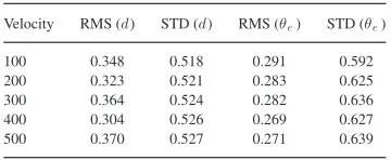
different velocitiesvranging from 100 pixels/s to 500 pixels/s with a step of 100. From Table V, it can be underlined that the accuracy remains very stable with a RMS ranging from 0.304 to 0.370 pixels fordand from 0.269 to 0.291 rad forθe, and STD within similar ranges.
F. CPU Load of the Controller
Note that in laser microphonosurgery, the laser scanning should works in high frequency, i.e., at least of 200 Hz (sam-pling time) to avoid tissue carbonization during tumors ablation or resection. As shown in Table VI, it can be noted that our
ap-100 0.348 0.518 0.291 0.592
200 0.323 0.521 0.283 0.625
300 0.364 0.524 0.282 0.636
400 0.304 0.526 0.269 0.627
500 0.370 0.527 0.271 0.639
TABLE VI
CPU LOAD OF THEMAINTASKS OF THEPROCESS
Task Time (m s)
image grabbing 0.064 laser tracking 0.471
controller 0.002
control sending (USB 2.0) 0.989
other 0.176
entire process 1.702 (f=587 Hz)
proach takes only 1.702 milliseconds (ms), which is equivalent to a frequency of 587 Hz (sampling time) despite the use of a slow USB communication.
VI. CONCLUSION
In this paper, a vision-guided laser steering technique us-ing a path followus-ing approach was presented. To do this, we were inspired by the methods used in mobile robotic (unicy-cle kinematic model) in order to develop an efficient controller scheme by taking into account the fact that the path following and the velocity profile must be decoupled. Thus, the proposed controller was based on the use of the curvilinear representa-tion of the laser steering kinematic model more adapted to our problem.
Our developments were validated in simulation, as well as in an experimental setup, in different conditions of use
1) using various initial velocity inputs: step input (fixed laser velocity), sinusoidal inputs, and successive steps inputs, 2) starting with large initial errors,
3) using low to high laser velocity (from 100 pixels/s to 500 pixels/s,
4) using optimized and nonoptimized parametersγ1andγ2,
5) using time-varying path (i.e.,Γ(t)) simulating a patient breathing,
6) using more complex curves with high curvatures (more complex comparing to the laser surgery paths).
re-peatability (more than 30 repetitions with the same order of accuracy), and frequency (587 Hz).
The next stages of this paper will involve adapting the de-scribed materials for real laser surgery applications, i.e., on a human cadaver using the entire endoscopic system developed in theµRALP project. In addition, the velocity will have to be servoed with regards to the heat profile in the tissue and to the depth variations of the tissues with respect to the image.
REFERENCES
[1] W. Schwesinger and J. Hunter, “Laser in general surgery, ”Surgical Clinics of North America. Philadelphia, PA, USA: Saunders, 1992.
[2] V. Moiseev, “Laser technologies in microsurgery of extramedullary tu-mors,” in Proc. Int. Conf. Actual Problems Elect. Inst. Eng., 2004, pp. 275–275.
[3] H. Eckel, S. Berendes, M. Damm, and J. Klusmann, “Suspension laryn-goscopy for endotracheal stenting,”Laryngoscope, vol. 113, pp. 11–15, 2003.
[4] M. Remacle, “Laser-assisted microphonosurgery,” inSurgery of Larynx and Trachea. Berlin, Germany: Springer, 2010, pp. 51–56.
[5] L. I. Israel. (2014, Feb.). Digital acublade system. israel@online. [Online]. Available: http://www.surgical.lumenis.com
[6] J. Ortiz, L. Mattos, and D. Caldwell, “Smart devices in robot-assisted laser microsurgery: Towards ubiquitous tele-cooperation,” inProc. IEEE Int. Conf. Rob. Biomimetics, 2012, pp. S1721–1726.
[7] L. Mattos, D. Nikhil, G. Barresi, L. Gustani, and G. Pirreti, “A novel com-puterized surgeon-machine interface for robot-assisted laser phonomicro-surgery,”Laryngoscope, vol. 124, pp. 1887–1894, 2014.
[8] T. Sibillano, A. Ancona, V. Berardi, and P. Lugar`a, “A real-time spec-troscopic sensor for monitoring laser welding processes,”Sensors, vol. 9, pp. 3376–3385, 2009.
[9] M. Fridenfalk and G. Bolmsjo, “Design and validation of a universal 6D seam-tracking system in robotic welding using arc sensing,”Adv. Robot., vol. 18, pp. 1–21, 2004.
[10] Y. Huang, Y. Xiao, P. Wang, and M. Li, “A seam-tracking laser welding platform with 3D and 2D visual information fusion vision sensor system,”
Int. J. Adv. Manuf. Technol., vol. 67, pp. 415–426, 2012.
[11] H. Cui, Z.Xiao, J. Dong; Y. Chen, G. Hou, and Z. Zhao, “Notice of retraction analysis on arc-welding robot visual control tracking system,” inProc. Int. Conf. Quality, Reliability, Risk, Maintain., Safety Eng., 2013, pp. 2091–2094.
[12] B. Thuilot, R. Lenain, P. Martinet, and C. Cariou, “Accurate GPS-based guidance of agricultural vehicles operating on slippery grounds,” inFocus on Robotics Research, John Liu ed., Commack, NY, USA: Nova, 2006, pp. 185–239.
[13] B. Thuilot, J. Bom, F. Marmoiton, and P. Martinet, “Accurate auto-matic guidance of an urban electric vehicle relying on a kineauto-matic GPS sensor,” in Proc. 5th IFAC Symp. Intel. Auton. Veh., Portugal, 2004, pp. 1–6.
[14] B. Petrak, K. Konthasinghe, S. Perez, and A. Muller, “Feedback-controlled laser fabrication of micromirror substrates,”Rev. Scient. Inst., vol. 82, no. 12, pp. 123112-1–123112-6, 2011.
[15] F. Arai, K. Yoshikawa, T. Sakami, and T. Fukuda, “Synchronized laser micromanipulation of multiple targets along each trajectory by single laser,”Appl. Phys. Lett., vol. 85, no. 19, pp. 4301–4303, 2004.
[16] R. W. Brockett, “Asymptotic stability and feedback stabilization,” in Dif-ferential Geometric Control Theory, Boston, MA, USA: Birkhauser, 1983, pp. 181–191.
[17] A. Bloch, M. Reyhanoglu, and N. McClamroch, “Control and stabilization of nonholonomic dynamic systems,”IEEE Trans. Autom. Control, vol. 37, no. 11, pp. 1746–1757, Nov. 1992.
[18] J. P. Hespanha, D. Liberzon, and A. Morse, “Logic-based switching control of a nonholonomic system with parametric modeling uncertainty,”Syst. Control Lett., vol. 38, no. 3, pp. 167–177, 1999.
[19] T. Floquet, J.-P. Barbot, and W. Perruquetti, “Higher-order sliding mode stabilization for a class of nonholonomic perturbed systems,”Automatica, vol. 39, no. 6, pp. 1077–1083, 2003.
[20] C. Samson, “Velocity and torque feedback control of a nonholonomic cart,” inAdvanced Robot Control. Berlin, Germany: Springer, 1991, vol. 162, pp. 125–151.
[21] M. Aicardi, G. Casalino, A. Bicchi, and A. Balestrino, “Closed loop steering of unicycle like vehicles via Lyapunov techniques,”IEEE Robot. Autom. Mag., vol. 2, no. 1, pp. 27–35, Mar. 1995.
[22] J. Godhavn and O. Egeland, “A Lyapunov approach to exponential sta-bilization of nonholonomic systems in power form,”IEEE Trans. Autom. Control., vol. 42, no. 7, pp. 1028–1032, Jul. 1997.
[23] C. Samson, “Mobile robot control. Part 2: Control of chained systems and application to path following and time-varying point stabilization of wheeled vehicles,” INRIA, Tech. Rep. 1994, 1993.
[24] P. Morin and C. Samson, “Motion control of wheeled mobile robots,” in
Springer Handbook of Robotics, B. Siciliano and O. Khatib, Eds. Berlin, Germany: Springer, 2008, pp. 799–826.
[25] E. Marchand, F. Spindler, and F. Chaumette, “Visp for visual servoing: A generic software platform with a wide class of robot control skills,”IEEE Robot. Autom. Mag., vol. 12, no. 4, pp. 40–52, Dec. 2005.
Jean-Antoine Seon received the Engineering de-gree in mechanical engineering and microtechnolo-gies from ENSMM, Besanc¸on, France, in 2013 and the Master’s degree in mechatronics and microsys-tems from Universit´e de Franche-Comt´e, Besanc¸on, France, in 2014. He is currently working toward the Ph.D degree with the AS2M Department, FEMTO-ST Institut, where his research is mainly focused on planning and control for dexterous micromanipula-tion.
Brahim Tamadaztereceived the Ph.D. degree in au-tomation and computer Sscience from “Universit´e de Franche-Comt´e,” Besanc¸on Cedex, France, in 2009 and the M.S. degree in robotics and intelligent sys-tems from “Universit´e Pierre et Marie Curie (Paris VI)” in 2005, France.
Since 2012 he has been with FEMTO-ST Institut, AS2M Department as Senior Scientist CNRS Re-searcher (Besanc¸on, France). He currently works in microrobotics surgery (conception and control) and visual servoing using an OCT imaging system.
Nicolas Andreffreceived the M.S. degree in com-puter sciences and applied mathematics from EN-SEEIHT, Toulouse, France, in 1994 and the Ph.D. degree in computer graphics, computer vision, and robotics from INPG, Grenoble, France, in 1999.