P H Y S I C S
Third edition
K e n n e t h S. K r a n e
D E P A R T M E N T O F P H Y S I C S
O R E G O N S T A T E U N I V E R S I T Y
CASSINI
INTERPLANETARY TRAJECTORY
VENUS SWINGBY 26 APR 1998
EARTH SWINGBY
18 AUG 1999 JUPITER SWINGBY 30 DEC 2000 VENUS SWINGBY
24 JUN 1999
LAUNCH 15 OCT 1997
ORBIT OF EARTH
ORBIT OF VENUS DEEP SPACE
MANEUVER 3 DEC 1990
ORBIT OF
JUPITER ORBIT OF
SATURN SATURN ARRIVAL
1 JUL 2004
THE FAILURES OF CLASSICAL
PHYSICS
If you were a physicist living at the end of the 19th century, you probably would have been pleased with the progress that physics had made in understanding the laws that govern the processes of nature. Newton’s laws of mechanics, including gravitation, had been carefully tested, and their success had provided a framework for understanding the interactions among objects. Electricity and magnetism had been unified by Maxwell’s theoretical work, and the electromagnetic waves predicted by Maxwell’s equations had been discovered and investigated in the experiments conducted by Hertz. The laws of thermodynamics and kinetic theory had been particularly successful in providing a unified explanation of a wide variety of phenomena involving heat and temperature. These three successful theories—mechanics, electromagnetism, and thermodynamics— form the basis for what we call “classical physics.”
Beyond your 19th-century physics laboratory, the world was undergoing rapid changes. The Industrial Revolution demanded laborers for the factories and accelerated the transition from a rural and agrarian to an urban society. These workers formed the core of an emerging middle class and a new economic order. The political world was changing, too—the rising tide of militarism, the forces of nationalism and revolution, and the gathering strength of Marxism would soon upset established governments. The fine arts were similarly in the middle of revolutionary change, as new ideas began to dominate the fields of painting, sculpture, and music. The understanding of even the very fundamental aspects of human behavior was subject to serious and critical modification by the Freudian psychologists.
In the world of physics, too, there were undercurrents that would soon cause revolutionary changes. Even though the overwhelming majority of experimental evidence agreed with classical physics, several experiments gave results that were not explainable in terms of the otherwise successful classical theories. Classical electromagnetic theory suggested that a medium is needed to propagate electro-magnetic waves, but precise experiments failed to detect this medium. Experiments to study the emission of electromagnetic waves by hot, glowing objects gave results that could not be explained by the classical theories of thermodynamics and electromagnetism. Experiments on the emission of electrons from surfaces illuminated with light also could not be understood using classical theories.
These few experiments may not seem significant, especially when viewed against the background of the many successful and well-understood experiments of the 19th century. However, these experiments were to have a profound and lasting effect, not only on the world of physics, but on all of science, on the political structure of our world, and on the way we view ourselves and our place in the universe. Within the short span of two decades between 1905 and 1925, the shortcomings of classical physics would lead to the special and general theories of relativity and the quantum theory.
The designationmodern physicsusually refers to the developments that began in about 1900 and led to the relativity and quantum theories, including the applications of those theories to understanding the atom, the atomic nucleus and the particles of which it is composed, collections of atoms in molecules and solids, and, on a cosmic scale, the origin and evolution of the universe. Our discussion of modern physics in this text touches on each of these areas.
physics offers either inadequate or incorrect conclusions. These situations are not necessarily those that originally gave rise to the relativity and quantum theories, but they do help us understand why classical physics fails to give us a complete picture of nature.
1.1 REVIEW OF CLASSICAL PHYSICS
Although there are many areas in which modern physics differs radically from classical physics, we frequently find the need to refer to concepts of classical physics. Here is a brief review of some of the concepts of classical physics that we may need.
Mechanics
A particle of massmmoving with velocityvhas akinetic energydefined by
K=12mv2 (1.1)
and alinear momentum
pdefined by
p=m
v (1.2)
In terms of the linear momentum, the kinetic energy can be written
K= p
2
2m (1.3)
When one particle collides with another, we analyze the collision by applying two fundamental conservation laws:
I. Conservation of Energy.The total energy of an isolated system (on which no net external force acts) remains constant. In the case of a collision between particles, this means that the total energy of the particlesbeforethe collision is equal to the total energy of the particlesafterthe collision.
II. Conservation of Linear Momentum. The total linear momentum of an isolated system remains constant. For the collision, the total linear momentum of the particlesbeforethe collision is equal to the total linear momentum of the particlesafterthe collision. Because linear momentum is a vector, application of this law usually gives us two equations, one for the xcomponents and another for theycomponents.
These two conservation laws are of the most basic importance to understanding and analyzing a wide variety of problems in classical physics. Problems 1–4 and 11–14 at the end of this chapter review the use of these laws.
Example 1.1
A helium atom (m=6.6465×10⁻²⁷kg) moving at a speed
ofvHe=1.518×10⁶m/s collides with an atom of
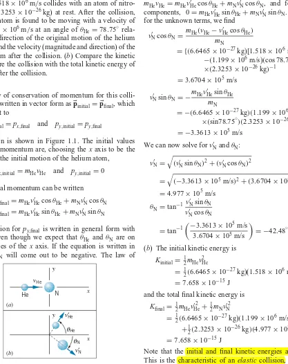
nitro-gen (m=2.3253×10⁻²⁶kg) at rest. After the collision, the helium atom is found to be moving with a velocity of v′He=1.199×10⁶m/s at an angle of θHe=78.75◦ rela-tive to the direction of the original motion of the helium atom. (a) Find the velocity (magnitude and direction) of the nitrogen atom after the collision. (b) Compare the kinetic energy before the collision with the total kinetic energy of the atoms after the collision.
Solution
(a) The law of conservation of momentum for this colli-sion can be written in vector form as
pinitial=pfinal, which is equivalent topx,initial=px,final and py,initial=py,final
The collision is shown in Figure 1.1. The initial values of the total momentum are, choosing thexaxis to be the direction of the initial motion of the helium atom,
px,initial=mHevHe and py,initial=0
The final total momentum can be written
px,final=mHev′HecosθHe+mNv′NcosθN py,final=mHev′HesinθHe+mNv′NsinθN
The expression forpy,final is written in general form with a+ sign even though we expect thatθHe andθN are on opposite sides of thexaxis. If the equation is written in this way, θN will come out to be negative. The law of
x
FIGURE 1.1 Example 1.1. (a) Before collision;
(b) after collision.
conservation of momentum gives, for thexcomponents, mHevHe=mHev′HecosθHe+mNv′NcosθN, and for the y components, 0=mHev′HesinθHe+mNv′NsinθN. Solving for the unknown terms, we find
v′NcosθN= mHe(vHe−v
(b) The initial kinetic energy is Kinitial=12mHev2 and the total final kinetic energy is
Kfinal= 12mHevHe′2 +12mNv′N2
Example 1.2
An atom of uranium (m=3.9529×10⁻²⁵kg) at rest
decays spontaneously into an atom of helium (m= 6.6465×10⁻²⁷kg) and an atom of thorium (m=3.8864× 10⁻²⁵kg). The helium atom is observed to move in the positive x direction with a velocity of 1.423×10⁷m/s
(Figure 1.2). (a) Find the velocity (magnitude and direc-tion) of the thorium atom. (b) Find the total kinetic energy of the two atoms after the decay.
x x
U
(a) (b)
Th He
v′Th v′He
y y
FIGURE 1.2 Example 1.2. (a) Before decay; (b) after decay.
Solution
(a) Here we again use the law of conservation of momen-tum. The initial momentum before the decay is zero, so the total momentum of the two atoms after the decay must also be zero:
px,initial=0 px,final =mHev′He+mThv′Th
Setting px,initial=px,final and solving forv′Th, we obtain
v′Th= −mHev′He
mTh
= −(6.6465×10−
27kg)(1.423×10⁷m/s)
3.8864×10⁻²⁵kg
= −2.432×10⁵m/s
The thorium atom moves in the negativexdirection.
(b) The total kinetic energy after the decay is:
K =12mHevHe′2 +12mThv′Th2
=1
2(6.6465×10⁻²⁷kg)(1.423×10⁷m/s)2
+1
2(3.8864×10−
25kg)(−2.432×10⁵m/s)2
=6.844×10⁻¹³J
Clearly kinetic energy is not conserved in this decay, because the initial kinetic energy of the uranium atom was zero. However total energy is conserved— if we write the total energy as the sum of kinetic energy and nuclear energy, then the total initial energy (kinetic + nuclear) is equal to the total final energy (kinetic + nuclear). Clearly the gain in kinetic energy occurs as a result of a loss in nuclear energy. This is an example of the type of radioactive decay called alpha decay, which we discuss in more detail in Chapter 12.
Another application of the principle of conservation of energy occurs when a particle moves subject to an external forceF. Corresponding to that external force there is often a potential energyU, defined such that (for one-dimensional motion)
F= −dU
dx (1.4)
The total energyEis the sum of the kinetic and potential energies:
E=K+U (1.5)
L = r× p
x
O y
z
p r
FIGURE 1.3 A particle of mass m,
located with respect to the origin O by position vector
r and moving with linear momentump, has angular momentumLaboutO.When a particle moving with linear momentum
pis at a displacementrfrom the originO, itsangular momentumLabout the pointOis defined (see Figure 1.3) byL=
r×p (1.6)There is a conservation law for angular momentum, just as with linear momentum. In practice this has many important applications. For example, when a charged particle moves near, and is deflected by, another charged particle, the total angular momentum of the system (the two particles) remains constant if no net external torque acts on the system. If the second particle is so much more massive than the first that its motion is essentially unchanged by the influence of the first particle, the angular momentum of the first particle remains constant (because the second particle acquires no angular momentum). Another application of the conservation of angular momentum occurs when a body such as a comet moves in the gravitational field of the Sun—the elliptical shape of the comet’s orbit is necessary to conserve angular momentum. In this case
rand
pof the comet must simultaneously change so thatLremains constant.
Velocity Addition
Another important aspect of classical physics is the rule for combining velocities. For example, suppose a jet plane is moving at a velocity of vPG=650 m/s, as measured by an observer on the ground. The subscripts on the velocity mean “velocity of the plane relative to the ground.” The plane fires a missile in the forward direction; the velocity of the missile relative to the plane is vMP=250 m/s. According to the observer on the ground, the velocity of the missile is:vMG=vMP+vPG=250 m/s+650 m/s=900 m/s.
We can generalize this rule as follows. Let
vAB represent the velocity of A relative toB, and letvBCrepresent the velocity ofBrelative toC. Then the velocity ofArelative toCisvAC=
vAB+vBC (1.7)This equation is written in vector form to allow for the possibility that the velocities might be in different directions; for example, the missile might be fired not in the direction of the plane’s velocity but in some other direction. This seems to be a very “common-sense” way of combining velocities, but we will see later in this chapter (and in more detail in Chapter 2) that this common-sense rule can lead to contradictions with observations when we apply it to speeds close to the speed of light.
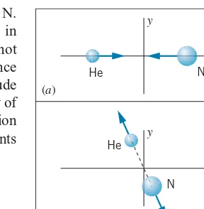
A common application of this rule (for speeds small compared with the speed of light) occurs in collisions, when we want to analyze conservation of momentum and energy in a frame of reference that is different from the one in which the collision is observed. For example, let’s analyze the collision of Example 1.1 in a frame of reference that is moving with the center of mass. Suppose the initial velocity of the He atom defines the positive x direction. The velocity of the center of mass (relative to the laboratory) is then vCL= (vHemHe+vNmN)/(mHe+mN)=3.374×105m/s. We would like to find the initial velocity of the He and N relative to the center of mass. If we start with vHeL=vHeC+vCLandvNL=vNC+vCL, then
vHeC=vHeL−vCL=1.518×10⁶m/s−3.374×105m/s=1.181×106m/s
In a similar fashion we can calculate the final velocities of the He and N. The resulting collision as viewed from this frame of reference is illustrated in Figure 1.4. There is a special symmetry in this view of the collision that is not apparent from the same collision viewed in the laboratory frame of reference (Figure 1.1); each velocity simply changes direction leaving its magnitude unchanged, and the atoms move in opposite directions. The angles in this view of the collision are different from those of Figure 1.1, because the velocity addition in this case applies only to the x components and leaves the y components unchanged, which means that the angles must change.
x
FIGURE 1.4 The collision of Figure
1.1 viewed from a frame of refer-ence moving with the center of mass. (a) Before collision. (b) After colli-sion. In this frame the two particles always move in opposite directions, and for elastic collisions the mag-nitude of each particle’s velocity is unchanged.
Electricity and Magnetism
The electrostatic force (Coulomb force) exerted by a charged particle q1 on another chargeq2has magnitude
F= 1 4πε0
|q1||q2|
r2 (1.8)
The direction ofF is along the line joining the particles (Figure 1.5). In the SI system of units, the constant 1/4πε0has the value
1
4πε0 =8.988×10
9
N·m2/C2
The corresponding potential energy is
U = 1 4πε0
q1q2
r (1.9)
In all equations derived from Eq. 1.8 or 1.9 as starting points,the quantity1/4πε0 must appear. In some texts and reference books, you may find electrostatic quantities in which this constant does not appear. In such cases, the centimeter-gram-second (cgs) system has probably been used, in which the constant 1/4πε0 isdefined to be 1. You should always be very careful in making comparisons of electrostatic quantities from different references and check that the units are identical.
r
+ +
F F
FIGURE 1.5 Two charged particles
experience equal and opposite elec-trostatic forces along the line joining their centers. If the charges have the same sign (both positive or both nega-tive), the force is repulsive; if the signs are different, the force is attractive. An electrostatic potential differenceVcan be established by a distribution of
charges. The most common example of a potential difference is that between the two terminals of a battery. When a chargeqmoves through a potential difference V, the change in its electrical potential energyUis
U=qV (1.10)
At the atomic or nuclear level, we usually measure charges in terms of the basic charge of the electron or proton, whose magnitude is e=1.602×10⁻¹⁹C. If
such charges are accelerated through a potential differenceVthat is a few volts, the resulting loss in potential energy and corresponding gain in kinetic energy will be of the order of 10−19to 10−18J. To avoid working with such small numbers, it is common in the realm of atomic or nuclear physics to measure energies in electron-volts(eV), defined to be the energy of a charge equal in magnitude to that of the electron that passes through a potential difference of 1 volt:
and thus
1 eV=1.602×10⁻¹⁹J
Some convenient multiples of the electron-volt are
keV=kilo electron-volt=103eV MeV=mega electron-volt=106eV
GeV=giga electron-volt=109eV
(In some older works you may find reference to the BeV, for billion electron-volts; this is a source of confusion, for in the United States a billion is 109 while in
Europe a billion is 1012.)
Often we wish to find the potential energy of two basic charges separated by typical atomic or nuclear dimensions, and we wish to have the result expressed in electron-volts. Here is a convenient way of doing this. First we express the quantitye2/4πε
0in a more convenient form:
e2
With this useful combination of constants it becomes very easy to calculate electrostatic potential energies. For two electrons separated by a typical atomic dimension of 1.00 nm, Eq. 1.9 gives
U = 1
For calculations at the nuclear level, the femtometer is a more convenient unit of distance and MeV is a more appropriate energy unit:
e2
It is remarkable (and convenient to remember) that the quantitye2/4πε
0 has the
same value of 1.440 whether we use typical atomic energies and sizes (eV·nm) or typical nuclear energies and sizes (MeV·fm).
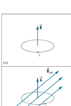
A magnetic fieldB
can be produced by an electric currenti. For example, the magnitude of the magnetic field at the center of a circular current loop of radiusr is (see Figure 1.6a)B= μ0i
2r (1.11)
The SI unit for magnetic field is the tesla (T), which is equivalent to a newton per ampere-meter. The constantμ0is
μ0=4π×10−7N·s2/C2
FIGURE 1.6 (a) A circular current
loop produces a magnetic field
B at its center. (b) A current loop with magnetic moment µ in an externalmagnetic field B
ext. The field exertsa torque on the loop that will tend to rotate it so thatµ
lines up withBext.thumb pointing in the direction of the current, the fingers point in the direction of the magnetic field.
It is often convenient to define themagnetic momentµ
of a current loop:
|µ
| =iA (1.12)where A is the geometrical area enclosed by the loop. The direction of µ
isperpendicular to the plane of the loop, according to the right-hand rule.
When a current loop is placed in a uniformexternalmagnetic fieldB
ext(as in Figure 1.6b), there is a torqueτon the loop that tends to line upµwithBext: τ=µ×Bext (1.13)
Another way to describe this interaction is to assign a potential energy to the magnetic momentµ
in the external fieldBext:U = −µ
·Bext (1.14)When the fieldB
ext is applied,µrotates so that its energy tends to a minimum
value, which occurs whenµ
andBextare parallel.
It is important for us to understand the properties of magnetic moments, because particles such as electrons or protons have magnetic moments. Although we don’t imagine these particles to be tiny current loops, their magnetic moments do obey Eqs. 1.13 and 1.14.
A particularly important aspect of electromagnetism iselectromagnetic waves. In Chapter 3 we discuss some properties of these waves in more detail. Electro-magnetic waves travel in free space with speedc(the speed of light), which is related to the electromagnetic constantsε0andμ0:
c=(ε0μ0)−1/2 (1.15)
The speed of light has the exact value ofc=299,792,458 m/s.
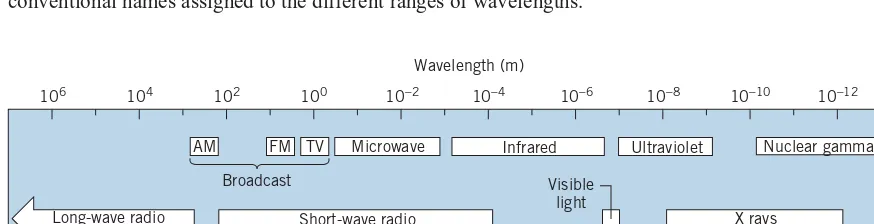
Electromagnetic waves have a frequency f and wavelength λ, which are related by
c=λf (1.16)
The wavelengths range from the very short (nuclear gamma rays) to the very long (radio waves). Figure 1.7 shows the electromagnetic spectrum with the conventional names assigned to the different ranges of wavelengths.
106 104 102 100 10−2 10−4 10−6 10−8 10−10 10−12
Frequency (Hz) Wavelength (m)
AM
102 104 106 108 1010 1012 1014 1016 1018 1020 1022
FM
Broadcast Visible
light
TV Microwave Infrared Ultraviolet
X rays Short-wave radio
Long-wave radio
Nuclear gamma rays
Kinetic Theory of Matter
An example of the successful application of classical physics to the structure of matter is the understanding of the properties of gases at relatively low pressures and high temperatures (so that the gas is far from the region of pressure and temperature where it might begin to condense into a liquid). Under these conditions, most real gases can be modeled as ideal gases and are well described by theideal gas equation of state
PV =NkT (1.17)
wherePis the pressure,Vis the volume occupied by the gas,Nis the number of molecules,T is the temperature, andkis theBoltzmann constant, which has the value
k=1.381×10⁻²³J/K
In using this equation and most of the equations in this section, the temperature must be measured in units of kelvins (K). Be careful not to confuse the symbol K for the unit of temperature with the symbolKfor kinetic energy.
The ideal gas equation of state can also be expressed as
PV =nRT (1.18)
where n is the number of moles and R is the universal gas constant with a value of
R=8.315 J/mol·K
One mole of a gas is the quantity that contains a number of fundamental entities (atoms or molecules) equal to Avogadro’s constantNA, where
NA=6.022×10²³per mole
That is, one mole of helium contains NA atoms of He, one mole of nitrogen contains NA molecules of N2 (and thus 2NA atoms of N), and one mole of
water vapor contains NA molecules of H2O (and thus 2NA atoms of H andNA atoms of O).
Because N=nNA (number of molecules equals number of moles times number of molecules per mole), the relationship between the Boltzmann constant and the universal gas constant is
R=kNA (1.19)
Individual molecules may speed up or slow down due to collisions, but the average kinetic energy of all the molecules in the container does not change. The average kinetic energy of a molecule in fact depends only on the temperature:
Kav= 32kT(per molecule) (1.20)
For rough estimates, the quantitykT is often used as a measure of the mean kinetic energy per particle. For example, at room temperature (20◦C=293 K), the mean kinetic energy per particle is approximately 4×10⁻²¹J (about 1/40 eV),
while in the interior of a star whereT ∼107K, the mean energy is approximately
10−16J (about 1000 eV).
Sometimes it is also useful to discuss the average kinetic energy of a mole of the gas:
averageKper mole=averageKper molecule× number of molecules per mole
Using Eq. 1.19 to relate the Boltzmann constant to the universal gas constant, we find the average molar kinetic energy to be
Kav= 32RT (per mole) (1.21)
It should be apparent from the context of the discussion whetherKavrefers to the average per molecule or the average per mole.
1.2 THE FAILURE OF CLASSICAL CONCEPTS
OF SPACE AND TIME
In 1905, Albert Einstein proposed the special theory of relativity, which is in essence a new way of looking at space and time, replacing the “classical” space and time that were the basis of the physical theories of Galileo and Newton. Einstein’s proposal was based on a “thought experiment,” but in subsequent years experimental data have clearly indicated that the classical concepts of space and time are incorrect. In this section we examine how experimental results support the need for a new approach to space and time.
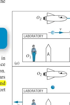
(a)
(b)
O2
O1 A
B
LABORATORY
v
O2
v
−v
O1 A
B
LABORATORY
FIGURE 1.8 (a) The pion experiment
according to O1. Markers A and B respectively show the locations of the pion’s creation and decay. (b) The same experiment as viewed by O2, relative to whom the pion is
at rest and the laboratory moves with velocity−v.
The Failure of the Classical Concept of Time
In high-energy collisions between two protons, many new particles can be produced, one of which is api meson(also known as apion). When the pions are produced at rest in the laboratory, they are observed to have an average lifetime (the time between the production of the pion and its decay into other particles) of 26.0 ns (nanoseconds, or 10−9s). On the other hand, pions in motion are observed to have a very different lifetime. In one particular experiment, pions moving at a speed of 2.737×10⁸m/s (91.3% of the speed of light) showed a lifetime of 63.7 ns.
lifetime to be 63.7 ns. Observer #2 is moving relative to the laboratory at exactly the same velocity as the pion, so according to observer #2 the pion is at rest and has a lifetime of 26.0 ns. The two observers measure different values for the time interval between the same two events—the formation of the pion and its decay.
According to Newton, time is the same for all observers. Newton’s laws are based on this assumption. The pion experiment clearly shows that time is not the same for all observers, which indicates the need for a new theory that relates time intervals measured by different observers who are in motion with respect to each other.
The Failure of the Classical Concept of Space
The pion experiment also leads to a failure of the classical ideas about space. Suppose observer #1 erects two markers in the laboratory, one where the pion is created and another where it decays. The distance D1 between the two markers is equal to the speed of the pion multiplied by the time interval from its creation to its decay: D1 =(2.737×10⁸m/s)(63.7×10−9s)=17.4 m. To observer #2, traveling at the same velocity as the pion, the laboratory appears to be rushing by at a speed of 2.737×10⁸m/s and the time between passing the first and second markers, showing the creation and decay of the pion in the laboratory, is 26.0 ns. According to observer #2, the distance between the markers isD2 =(2.737×10⁸m/s)(26.0×10−9s)=7.11 m. Once again, we have two observers in relative motion measuring different values for the same interval, in this case the distance between the two markers in the laboratory. The physical theories of Galileo and Newton are based on the assumption that space is the same for all observers, and so length measurements should not depend on relative motion. The pion experiment again shows that this cornerstone of classical physics is not consistent with modern experimental data.
The Failure of the Classical Concept of Velocity
Classical physics places no limit on the maximum velocity that a particle can reach. One of the basic equations of kinematics, v=v0+at, shows that if a
particle experiences an accelerationafor a long enough timet, velocities as large as desired can be achieved, perhaps even exceeding the speed of light. For another example, when an aircraft flying at a speed of 200 m/s relative to an observer on the ground launches a missile at a speed of 250 m/s relative to the aircraft, a ground-based observer would measure the missile to travel at a speed of 200 m/s+ 250 m/s = 450 m/s, according to the classical velocity addition rule (Eq. 1.7). We can apply that same reasoning to a spaceship moving at a speed of 2.0×10⁸m/s
(relative to an observer on a space station), which fires a missile at a speed of 2.5×10⁸m/s relative to the spacecraft. We would expect that the observer on the space station would measure a speed of 4.5×10⁸m/s for the missile. This speed exceeds the speed of light (3.0×10⁸m/s). Allowing speeds greater than
the speed of light leads to a number of conceptual and logical difficulties, such as the reversal of the normal order of cause and effect for some observers.
Here again modern experimental results disagree with the classical ideas. Let’s go back again to our experiment with the pion, which is moving through the laboratory at a speed of 2.737×10⁸m/s. The pion decays into another particle,
a velocity of 2.737×10⁸m/s+0.813×108m/s=3.550×108m/s, exceeding
the speed of light. The observed velocity of the muon, however, is 2.846× 10⁸m/s, below the speed of light. Clearly the classical rule for velocity addition fails in this experiment.
The properties of time and space and the rules for combining velocities are essential concepts of the classical physics of Newton. These concepts are derived from observations at low speeds, which were the only speeds available to Newton and his contemporaries. In Chapter 2, we shall discover how the special theory of relativity provides the correct procedure for comparing measurements of time, distance, and velocity by different observers and thereby removes the failures of classical physics at high speed (while reducing to the classical laws at low speed, where we know the Newtonian framework works very well).
1.3 THE FAILURE OF THE CLASSICAL THEORY
OF PARTICLE STATISTICS
Thermodynamics and statistical mechanics were among the great triumphs of 19th-century physics. Describing the behavior of complex systems of many particles was shown to be possible using a small number of aggregate or average properties—for example, temperature, pressure, and heat capacity. Perhaps the crowning achievement in this field was the development of relationships between macroscopicproperties, such as temperature, andmicroscopicproperties, such as the molecular kinetic energy.
Despite these great successes, this statistical approach to understanding the behavior of gases and solids also showed a spectacular failure. Although the classical theory gave the correct heat capacities of gases at high temperatures, it failed miserably for many gases at low temperatures. In this section we summarize the classical theory and explain how it fails at low temperatures. This failure directly shows the inadequacy of classical physics and the need for an approach based on quantum theory, the second of the great theories of modern physics.
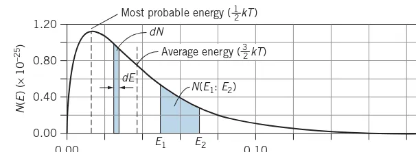
The Distribution of Molecular Energies
In addition to the average kinetic energy, it is also important to analyze the distribution of kinetic energies—that is, what fraction of the molecules in the container has kinetic energies between any two valuesK1 andK2. For a gas in thermal equilibrium at absolute temperature T (in kelvins), the distribution of molecular energies is given by theMaxwell-Boltzmann distribution:
N(E)= √2N π
1 (kT)3/2E
1/2e−E/kT (1.22)
In this equation,Nis the total number of molecules (a pure number) whileN(E) is the distribution function (with units of energy−1)defined so thatN(E)dEis the
number of moleculesdN in the energy intervaldEatE(or, in other words, the number of molecules with energies betweenEandE+dE):
dN =N(E)dE (1.23)
0.00
FIGURE 1.9 The Maxwell-Boltzmann energy distribution function, shown for
one mole of gas at room temperature (300 K).
axis into an infinite number of such small intervals and add the areas of all the resulting narrow strips, we obtain the total number of molecules in the gas:
∞ which you can find in tables of integrals. Also using calculus techniques (see Problem 8), you can show that the peak of the distribution function (the most probable energy) is 12kT.
The average energy in this distribution of molecules can also be found by dividing the distribution into strips. To find the contribution of each strip to the energy of the gas, we multiply the number of molecules in each strip, dN =N(E)dE, by the energyEof the molecules in that strip, and then we add the contributions of all the strips by integrating over all energies. This calculation would give thetotalenergy of the gas; to find the average we divide by the total number of moleculesN:
Once again, the definite integral can be found in integral tables. The result of carrying out the integration is
Eav=32kT (1.26)
Equation 1.26 gives the average energy of a molecule in the gas and agrees precisely with the result given by Eq. 1.20 for the ideal gas in which kinetic energy is the only kind of energy the gas can have.
Occasionally we are interested in finding the number of molecules in our distribution with energies between any two values E1 and E2. If the interval betweenE1andE2is very small, Eq. 1.23 can be used, withdE=E2−E1and with
N(E)evaluated at the midpoint of the interval. This approximation works very well when the interval is small enough thatN(E)is either approximately flat or linear over the interval. If the interval is large enough that this approximation is not valid, then it is necessary to integrate to find the number of molecules in the interval:
N(E1 :E2)=
Example 1.3
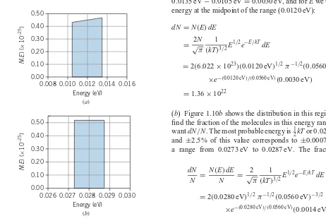
(a) In one mole of a gas at a temperature of 650 K(kT = 8.97×10⁻²¹J=0.0560 eV), calculate the number of molecules with energies between 0.0105 eV and 0.0135 eV. (b) In this gas, calculate the fraction of the molecules with energies in the range of ±2.5% of the most probable energy (12kT).
0.026 0.027 0.028 0.029 0.030
Energy (eV) graph is very close to linear in this region, we can use Eq. 1.23 to find the number of molecules in this range. We take dE to be the width of the range, dE=E2−E1= 0.0135 eV−0.0105 eV=0.0030 eV, and forEwe use the energy at the midpoint of the range (0.0120 eV):
dN =N(E)dE
(b) Figure 1.10bshows the distribution in this region. To find the fraction of the molecules in this energy range, we wantdN/N. The most probable energy is12kTor 0.0280 eV,
Note thatN(E)has dimensions of energy−1—it gives the number of molecules
per unit energy interval(for example, number of molecules per eV). To get an actual number that can be compared with measurement,N(E)must be multiplied by an energy interval. In our study of modern physics, we will encounter many different types of distribution functions whose use and interpretation are similar to that of N(E). These functions generally give a number or a probability per some sort of unit interval (for example, probability per unit volume), and to use the distribution function to calculate an outcome we must always multiply by an appropriate interval (for example, an element of volume). Sometimes we will be able to deal with small intervals using a relationship similar to Eq. 1.23, as we did in Example 1.3, but in other cases we will find the need to evaluate an integral, as we did in Eq. 1.27.
Polyatomic Molecules and the Equipartition of Energy
So far we have been considering gases with only one atom per molecule (monatomic gases). For “point” molecules with no internal structure, only one form of energy is important: translational kinetic energy 12mv2. (We call this “translational” kinetic energy because it describes motion as the gas particles move from one location to another. Soon we will also consider rotational kinetic energy.)
Let’s rewrite Eq. 1.26 in a more instructive form by recognizing that, with translational kinetic energy as the only form of energy, E=K= 12mv2. With
v2=v2
x+v2y+v2z, we can write the energy as
E= 1 2mv
2
x+12mv
2
y+12mv
2
z (1.28)
The average energy is then
1 2m(v
2
x)av+12m(v
2
y)av+12m(v
2
z)av= 32kT (1.29)
For a gas molecule there is no difference between thex,y, andzdirections, so the three terms on the left are equal and each term is equal to 12kT. The three terms on the left represent threeindependentcontributions to the energy of the molecule— the motion in thexdirection, for example, is not affected by theyor zmotions.
We define adegree of freedomof the gas as each independent contribution to the energy of a molecule, corresponding to one quadratic term in the expression for the energy. There are three quadratic terms in Eq. 1.28, so in this case there are three degrees of freedom. As you can see from Eq. 1.29, each of the three degrees of freedom of a gas molecule contributes an energy of 12kTto its average energy. The relationship we have obtained in this special case is an example of the application of a general theorem, called theequipartition of energy theorem:
When the number of particles in a system is large and Newtonian mechanics is obeyed, each molecular degree of freedom corresponds to an average energy of 12kT .
The average energy per molecule is then the number of degrees of freedom times
1
molecule by the number of moleculesN:Etotal=NEav. We will refer to this total
energy as theinternal energy Eintto indicate that it represents the random motions
of the gas molecules (in contrast, for example, to the energy involved with the motion of the entire container of gas molecules).
Eint=N(32kT)= 3 2NkT=
3
2nRT (translation only) (1.30)
where Eq. 1.19 has been used to express Eq. 1.30 in terms of either the number of molecules or the number of moles.
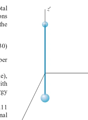
The situation is different for a diatomic gas (two atoms per molecule), illustrated in Figure 1.11. There are still three degrees of freedom associated with the translational motion of the molecule, but now two additional forms of energy are permitted—rotational and vibrational.
x′
y′
z′
FIGURE 1.11 A diatomic molecule,
with the origin at the center of mass. Rotations can occur about thex′andy′ axes, and vibrations can occur along thez′axis.
First we consider the rotational motion. The molecule shown in Figure 1.11 can rotate about thex′andy′axes (but not about thez′axis, because the rotational inertia about that axis is zero for diatomic molecules in which the atoms are treated as points). Using the general form of 12Iω2 for the rotational kinetic energy, we
can write the energy of the molecule as
E= 12mv2
x+12mv2y+12mvz2+12Ix′ω2x′+
1
2Iy′ωy2′ (1.31)
Here we have 5 quadratic terms in the energy, and thus 5 degrees of freedom. According to the equipartition theorem, the average total energy per molecule is 5×12kT = 52kT, and the total internal energy ofnmoles of the gas is
Eint =52nRT (translation + rotation) (1.32)
If the molecule can also vibrate, we can imagine the rigid rod connecting the atoms in Figure 1.11 to be replaced by a spring. The two atoms can then vibrate in opposite directions along thez′ axis, with the center of mass of the molecule remaining fixed. The vibrational motion adds two quadratic terms to the energy, corresponding to the vibrational potential energy (12kz′2) and the vibrational kinetic energy (12mv2
z′). Including the vibrational motion, there are now 7 degrees of freedom, so that
Eint=72nRT (translation + rotation + vibration) (1.33)
Heat Capacities of an Ideal Gas
Now we examine where the classical molecular distribution theory, which gives a very good accounting of molecular behavior under most circumstances, fails to agree with one particular class of experiments. Suppose we have a container of gas with a fixed volume. We transfer energy to the gas, perhaps by placing the container in contact with a system at a higher temperature. All of this transferred energy increases the internal energy of the gas by an amountEint, and there is an accompanying increase in temperatureT.
We define themolar heat capacityfor this constant-volume process as
CV = Eint
nT (1.34)
CV = 32R (monatomic or nonrotating, nonvibrating diatomic ideal gas) CV = 52R (rotating diatomic ideal gas) (1.35)
CV = 72R (rotating and vibrating diatomic ideal gas)
When we add energy to the gas, the equipartition theorem tells us that the added energy will on the average be distributed uniformly among all the possible forms of energy (corresponding to the number of degrees of freedom). However,only the translational kinetic energy contributes to the temperature(as shown by Eqs. 1.20 and 1.21). Thus, if we add 7 units of energy to a diatomic gas with rotating and vibrating molecules, on the average only 3 units go into translational kinetic energy and so 3/7 of the added energy goes into increasing the temperature. (To measure the temperature rise, the gas molecules must collide with the thermometer, so energy in the rotational and vibrational motions is not recorded by the thermometer.) Put another way, to obtain the same temperature increase T, a mole of diatomic gas requires 7/3 times the energy that is needed for a mole of monatomic gas.
Comparison with Experiment
How well do these heat capacity valuesagree with experiment? For monatomic gases, the agreement is very good. The equipartition theorem predicts a value of CV =3R/2=12.5 J/mol·K, which should be the same for all monatomic gases and the same at all temperatures (as long as the conditions of the ideal gas model are fulfilled). The heat capacity of He gas is 12.5 J/mol·K at 100 K, 300 K (room temperature), and 1000 K, so in this case our calculation is in perfect agreement with experiment. Other inert gases (Ne, Ar, Xe, etc.) have identical values, as do vapors of metals (Cu, Na, Pb, Bi, etc.) and the monatomic (dissociated) state of elements that normally form diatomic molecules (H, N, O, Cl, Br, etc.). So over a wide variety of different elements and a wide range of temperatures, classical statistical mechanics is in excellent agreement with experiment.
The situation is much less satisfactory for diatomic molecules. For a rotating and vibrating diatomic molecule, the classical calculation gives CV =7R/2=
29.1 J/mol·K. Table 1.1 shows some values of the heat capacities for different diatomic gases over a range of temperatures.
TABLE 1.1 Heat Capacities of Diatomic Gases
CV (J/mol·K)
Element 100 K 300 K 1000 K
H2 18.7 20.5 21.9
N2 20.8 20.8 24.4
O2 20.8 21.1 26.5
F2 20.8 23.0 28.8
Cl2 21.0 25.6 29.1
Br2 22.6 27.8 29.5
I2 24.8 28.6 29.7
Sb2 28.1 29.0
Te2 28.2 29.0
At high temperatures, many of the diatomic gases do indeed approach the expected value of 7R/2, but at lower temperatures the values are much smaller. For example, fluorine seems to behave as if it has 5 degrees of freedom (CV=20.8 J/mol·K) at 100 K and 7 degrees of freedom (CV=29.1 J/mol·K) at 1000 K.
Hydrogen behaves as if it has 5 degrees of freedom at room temperature, but at high enough temperature (3000 K), the heat capacity of H2 approaches 29.1 J/mol·K, corresponding to 7 degrees of freedom, while at lower temperatures (40 K) the heat capacity is 12.5 J/mol·K, corresponding to 3 degrees of freedom. The temperature dependence of the heat capacity of H2is shown in Figure 1.12.
There are three plateaus in the graph, corresponding to heat capacities for 3, 5, and 7 degrees of freedom. At the lowest temperatures, the rotational and vibrational motions are “frozen” and do not contribute to the heat capacity. At about 100 K, the molecules have enough energy to allow rotational motion to occur, and by about 300 K the heat capacity is characteristic of 5 degrees of freedom. Starting about 1000 K, the vibrational motion can occur, and by about 3000 K there are enough molecules above the vibrational threshold to allow 7 degrees of freedom. What’s going on here? The classical calculation demands thatCV should be constant, independent of the type of gas or the temperature. The equipartition of energy theorem, which is very successful in predicting many thermodynamic properties, fails miserably in accounting for the heat capacities. This theorem requires that the energy added to a gas must on average be divided equally among all the different forms of energy, and classical physics does not permit a threshold energy for any particular type of motion. How is it possible for 2 degrees of freedom, corresponding to the rotational or vibrational motions, to be “turned on” as the temperature is increased?
The solution to this dilemma can be found inquantum mechanics, according to which there is indeed a minimum or threshold energy for the rotational and vibrational motions. We discuss this behavior in Chapters 5 and 9. In Chapter 11 we discuss the failure of the equipartition theorem to account for the heat capacities of solids and the corresponding need to replace the classical Maxwell-Boltzmann energy distribution function with a different distribution that is consistent with quantum mechanics.
10 12.5 20.8
Cv
(J/mol
. K) 29.1
25 50 100 250 500 2500
Temperature (K)
5000 1000
Classical Prediction
Translation
Rotation
Vibration R 7 2
R 5 2
R 3 2
FIGURE 1.12 The heat capacity of molecular hydrogen at different temperatures.
1.4 THEORY, EXPERIMENT, LAW
When you first began to study science, perhaps in your elementary or high school years, you may have learned about the “scientific method,” which was supposed to be a sort of procedure by which scientific progress was achieved. The basic idea of the “scientific method” was that, on reflecting over some particular aspect of nature, the scientist would invent ahypothesisortheory,which would then be tested byexperimentand if successful would be elevated to the status oflaw. This procedure is meant to emphasize the importance of doing experiments as a way of testing hypotheses and rejecting those that do not pass the tests. For example, the ancient Greeks had some rather definite ideas about the motion of objects, such as projectiles, in the Earth’s gravity. Yet they tested none of these by experiment, so convinced were they that the power of logical deductionalonecould be used to discover the hidden and mysterious laws of nature and that once logic had been applied to understanding a problem, no experiments were necessary. If theory and experiment were to disagree, they would argue, then there must be something wrong with the experiment! This dominance of analysis and faith was so pervasive that it was another 2000 years before Galileo, using an inclined plane and a crude timer (equipment surely within the abilities of the early Greeks to construct), dis-covered the laws of motion, which were later organized and analyzed by Newton. In the case of modern physics, none of the fundamental concepts is obvious from reason alone. Only by doing often difficult and necessarily precise experi-ments do we learn about these unexpected and fascinating effects associated with such modern physics topics as relativity and quantum physics. These experiments have been done to unprecedented levels of precision—of the order of one part in 106 or better—and it can certainly be concluded that modern physics was tested far better in the 20th century than classical physics was tested in all of the preceding centuries.
Nevertheless, there is a persistent and often perplexing problem associated with modern physics, one that stems directly from your previous acquaintance with the “scientific method.” This concerns the use of the word “theory,” as in “theory of relativity” or “quantum theory,” or even “atomic theory” or “theory of evolution.” There are two contrasting and conflicting definitions of the word “theory” in the dictionary:
1. A hypothesis or guess.
2. An organized body of facts or explanations.
The “scientific method” refers to the first kind of “theory,” while when we speak of the “theory of relativity” we refer to the second kind. Yet there is often confusion between the two definitions, and therefore relativity and quantum physics are sometimes incorrectly regarded as mere hypotheses, on which evidence is still being gathered, in the hope of someday submitting that evidence to some sort of international (or intergalactic) tribunal, which in turn might elevate the “theory” into a “law.” Thus the “theory of relativity” might someday become the “law of relativity,” like the “law of gravity.”Nothing could be further from the truth!
experimental evidence for all of these processes is so compelling that no one who approaches them in the spirit of free and open inquiry can doubt the observational evidence or their inferences. Whether these collections of evidence are called theories or laws is merely a question of semantics and has nothing to do with their scientific merits. Like all scientific principles, they will continue to develop and change as new discoveries are made; that is the essence of scientific progress.
Chapter Summary
In an isolated system, the energy, linear momentum, and
Energy per degree of freedom = 12kT
1.3
Questions
1. Under what conditions can you apply the law of conservation of energy? Conservation of linear momentum? Conservation of angular momentum?
2. Which of the conserved quantities are scalars and which are vectors? Is there a difference in how we apply conservation laws for scalar and vector quantities?
3. What other conserved quantities (besides energy, linear momentum, and angular momentum) can you name?
4. What is the difference between potential and potential energy? Do they have different dimensions? Different units?
5. In Section 1.1 we defined the electric force between two charges and the magnetic field of a current. Use these quan-tities to define the electric field of a single charge and the magnetic force on a moving electric charge.
6. Other than from the ranges of wavelengths shown in Figure 1.7, can you think of a way to distinguish radio waves from infrared waves? Visible from infrared? That is,
could you design a radio that could be tuned to infrared waves? Could living beings “see” in the infrared region?
7. Suppose we have a mixture of an equal number N of molecules of two different gases, whose molecular masses arem1andm2, in complete thermal equilibrium at tempera-tureT. How do the distributions of molecular energies of the two gases compare? How do their average kinetic energies per molecule compare?
8. In most gases (as in the case of hydrogen) the rotational motion begins to occur at a temperature well below the temperature at which vibrational motion occurs. What does this tell us about the properties of the gas molecules?
10. At low temperatures the molar heat capacity of carbon diox-ide (CO2) is about 5R/2, and it rises to about 7R/2 at room temperature. However, unlike the gases discussed in Section 1.3, the heat capacity of CO2continues to rise as the temperature increases, reaching 11R/2 at 1000 K. How can you explain this behavior?
11. If we double the temperature of a gas, is the number of molecules in a narrow intervaldEaround the most probable energy about the same, double, or half what it was at the original temperature?
Problems
1.1 Review of Classical Physics
1. A hydrogen atom (m=1.674×10⁻²⁷kg) is moving with
a velocity of 1.1250×10⁷m/s. It collides elastically with
a helium atom (m=6.646×10⁻²⁷kg) at rest. After the
collision, the hydrogen atom is found to be moving with a velocity of−6.724×10⁶m/s (in a direction opposite to its original motion). Find the velocity of the helium atom after the collision in two different ways: (a) by applying conservation of momentum; (b) by applying conservation of energy.
2. A helium atom (m=6.6465×10⁻²⁷kg) collides elastically
with an oxygen atom (m=2.6560×10⁻²⁶kg) at rest. After
the collision, the helium atom is observed to be moving with a velocity of 6.636×10⁶m/s in a direction at an angle of
84.7◦relative to its original direction. The oxygen atom is observed to move at an angle of−40.4◦. (a) Find the speed of the oxygen atom. (b) Find the speed of the helium atom before the collision.
3. A beam of helium-3 atoms (m=3.016 u) is incident on a target of nitrogen-14 atoms (m=14.003 u) at rest. During the collision, a proton from the helium-3 nucleus passes to the nitrogen nucleus, so that following the collision there are two atoms: an atom of “heavy hydrogen” (deuterium,
m=2.014 u) and an atom of oxygen-15 (m=15.003 u). The incident helium atoms are moving at a velocity of 6.346×10⁶m/s. After the collision, the deuterium atoms
are observed to be moving forward (in the same direction as the initial helium atoms) with a velocity of 1.531×10⁷m/s.
(a) What is the final velocity of the oxygen-15 atoms? (b) Compare the total kinetic energies before and after the collision.
4. An atom of beryllium (m=8.00 u) splits into two atoms of helium (m=4.00 u) with the release of 92.2 keV of energy. If the original beryllium atom is at rest, find the kinetic energies and speeds of the two helium atoms.
5. A 4.15-volt battery is connected across a parallel-plate capacitor. Illuminating the plates with ultraviolet light causes electrons to be emitted from the plates with a speed of 1.76×10⁶m/s. (a) Suppose electrons are emitted near the center of the negative plate and travel perpendicular to that plate toward the opposite plate. Find the speed of the elec-trons when they reach the positive plate. (b) Suppose instead
that electrons are emitted perpendicular to the positive plate. Find their speed when they reach the negative plate.
1.2 The Failure of Classical Concepts of Space and Time
6. Observer A, who is at rest in the laboratory, is studying a particle that is moving through the laboratory at a speed of 0.624cand determines its lifetime to be 159 ns. (a) Observer A places markers in the laboratory at the locations where the particle is produced and where it decays. How far apart are those markers in the laboratory? (b) Observer B, who is traveling parallel to the particle at a speed of 0.624c, observes the particle to be at rest and measures its lifetime to be 124 ns. According to B, how far apart are the two markers in the laboratory?
1.3 The Failure of the Classical Theory of Particle Statistics
7. A sample of argon gas is in a container at 35.0◦C and 1.22 atm pressure. The radius of an argon atom (assumed spherical) is 0.710×10⁻¹⁰m. Calculate the fraction of the container volume actually occupied by the atoms.
8. By differentiating the expression for the Maxwell-Boltzmann energy distribution, show that the peak of the distribution occurs at an energy of 12kT.
9. A container holdsNmolecules of nitrogen gas atT=280 K. Find the number of molecules with kinetic energies between 0.0300 eV and 0.0312 eV.
10. A sample of 2.37 moles of an ideal diatomic gas experi-ences a temperature increase of 65.2 K at constant volume. (a) Find the increase in internal energy if only translational and rotational motions are possible. (b) Find the increase in internal energy if translational, rotational, and vibrational motions are possible. (c) How much of the energy calculated in (a) and (b) is translational kinetic energy?
General Problems
11. An atom of massm1=mmoving in thex direction with speed v1=v collides elastically with an atom of mass
m2=3mat rest. After the collision the first atom moves in theydirection. Find the direction of motion of the second atom and the speeds of both atoms (in terms ofv) after the collision.
massm2=2mmoving in the positiveydirection with speed
v2=2v/3. Find the resultant speed and direction of motion of the combination, and find the kinetic energy lost in this inelastic collision.
13. Suppose the beryllium atom of Problem 4 were not at rest, but instead moved in the positive x direction and had a kinetic energy of 40.0 keV. One of the helium atoms is found to be moving in the positive x direction. Find the direction of motion of the second helium, and find the veloc-ity of each of the two helium atoms. Solve this problem in two different ways: (a) by direct application of conservation of momentum and energy; (b) by applying the results of Problem 4 to a frame of reference moving with the original beryllium atom and then switching to the reference frame in which the beryllium is moving.
14. Suppose the beryllium atom of Problem 4 moves in the posi-tivexdirection and has kinetic energy 60.0 keV. One helium atom is found to move at an angle of 30◦with respect to the
xaxis. Find the direction of motion of the second helium atom and find the velocity of each helium atom. Work this
problem in two ways as you did the previous problem. (Hint:
Consider one helium to be emitted with velocity components
vxandvyin the beryllium rest frame. What is the relationship betweenvxandvy? How dovxandvychange when we move in thexdirection at speedv?)
15. A gas cylinder contains argon atoms (m=40.0 u). The tem-perature is increased from 293 K (20◦C) to 373 K (100◦C). (a) What is the change in the average kinetic energy per atom? (b) The container is resting on a table in the Earth’s gravity. Find the change in the vertical position of the con-tainer that produces the same change in the average energy per atom found in part (a).
16. Calculate the fraction of the molecules in a gas that are moving with translational kinetic energies between 0.02kT
and 0.04kT.
17. For a molecule of O2at room temperature (300 K), calculate the average angular velocity for rotations about thex′ory′