CALCULUS OF FINITE DIFFERENCES jordan

CALCULUS

O F

FINITE DIFFERENCES

BY

INTRODUCTION B Y

SECOND EDITION

CHELSEA PUBLISHING COMPANY

NEW YORK, N.Y.

I N T R O D U C T I O N

There is more than mere coincidence in the fact that the recent rapid growth in the theory and application of mathema-tical statistics has been accompanied by a revival in interest in the Calculus of Finite Differences. The reason for this pheno-mena is clear: the student of mathematical statistics must now regard the finite calculus as just as important a tool and pre-requisite as the infinitesimal calculus.

To my mind, the progress that has been made to date in the development of the finite calculus has been marked and stimulated by the of four outstanding texts.

The first of these was the treatise by George Boole that appeared in 1860. I do not by this to underestimate the valuable contributions of earlier writers on this subject or to overlook the elaborate work of I merely wish to state that Boole was the first to present’ this subject in a form best suited to the needs of student and teacher.

The second milestone was the remarkable work of

that appeared in 1924. This book presented the first rigorous treatment of the subject, and was written from the point of view of the mathematician rather the statistician. It was most oportune.

Steffensen’s

Interpolation,

the third of the four texts to which have referred, presents an excellent treatment of one section of the Calculus of Finite Differences, namely interpola-tion and summainterpola-tion formulae, and merits the commendainterpola-tion of both mathematicians and statisticians.

I do not hesitate to predict that the fourth of the texts that

Volume 3 of d u C a l c u l D i f f d r e n t i e l e t d u C a l c u l

v i

I have in mind, Professor Jordan’s Calculus of Finite Differen-ces, is destined to remain the classic treatment of this subject especially for statisticians for many years to come. Although an inspection of the table of contents reveals a coverage so extensive that the work of more than 600 pages might lead one at first to regard this book as an encyclopedia on the subject, yet a reading of any chapter of the text will impress the reader as a friendly lecture revealing an ununsual appreciation of both rigor and the computing technique so im-portant to the statistician.

The author has made a most thorough study of literature that has appeared during the last two centuries on the calculus of finite differences and has not hesitated in resurrecting for-gotten journal contributions and giving them the emphasis that his long experience indicates they deserve in this day of mathe-matical statistics.

In a word, Professor Jordan’s work is a most readable and detailed record of lectures on the Calculus of Finite Differences which will certainly appeal tremendously to the statistician and which could have been written only by one possessing a deep appreciation of mathematical statistics.

THE AUTHOR’S PREFACE

This book, a result of nineteen years’ lectures on the Cal-culus of Finite Differences, Probability, and Mathematical Sta-tistics in the Budapest University of Technical and Economical Sciences, and based on the venerable works of

Stirling, Euler

and has been written especially for practical use, with the object of shortening and facilitating the of the Com-puter. With this aim in view, some of the old and neglected, though useful, methods have been utilized and further developed: as for instance Stirling’s methods of summation,

Boole’s

symbo-lical methods, and

Laplace’s

method of Generating Functions, which last is especially helpful for the resolution of equations of partial differences,

The great practical value of

Newton’s

formula is shown; this is in general little appreciated by the Computer and the Statistician, who as a rule develop their functions in power series, although they are primarily concerned with the differences and sums of their functions, which in this case are hard to compute, but easy with the use of _-

Newton’s

_- formula. Even for interpolation more advisable to employ

Newton’s

expansion than to expand the function into a power series.

a great number of formulae is considerably shortened by using these numbers, and many new formulae are obtained by their aid; for instance, those which express differences by derivatives or vice formulae for the operations and and many others; formulae for the inversion of certain sums, for changing the length of the interval of the differences, for summation of reciprocal powers, etc.

In this book the functions especially useful in the Calculus of Finite Differences, such as the Factorial, the Binomial Coef-ficient, the Digamma and Trigamma Functions, and the Bernoulli and

Euler

Polynomials are fully treated. Moreover two species of polynomials, even more useful, analogous to those of Bernoulli and

Euler,

have been introduced; these are the

Bernoulli

nomiali of the second kind and the polynomials

Some new methods which permit great simplifications, will also be found, such as the method of interpolation without printed differences which reduces the cost and size of tables to a minimum. Though this formula has been especially deduced for Computers working with a calculating machine, it demands no more work of computation, even without this aid, than

Everett’s

formula, which involves the use of the even dif-ferences. Of course, if a table contains both the odd and the even differences, then interpolation by

Newton’s

formula is the shortest way, But there are very few tables which contain the first three differences, and hardly any with more than three, which would make the table too large and too expensive; moreover, the advantage of having the differences is not very . great, provided one works with a machine, as has been shown, even in the case of linear interpolation 133). So the printing of the differences may be considered as superfluous.

number of the decimals in the table, are given, then this deter-mines the range or the interval of the table. But generally, as is shown, the range chosen is ten or twenty times too large, or the interval as much too small; and the table is therefore unnecessarily bulky. If the table _{were reduced to the proper}

dimensions, it would be easy and very useful to add another table for the inverse function.

A method of approximation by aid of orthogonal polyno-mials, which greatly simplifies the operations, is given. Indeed, the orthogonal polynomials are used only temporarily, and the result obtained is expressed by Newton’s formula so

that no tables are necessary for giving the numerical values of the orthogonal polynomials.

In 143 an exceedingly simple method of graduation ac-cording to the principle of least squares is given, in which it is only necessary to compute certain “orthogonal” moments cor-responding to the data.

In the Chapter dealing with the numerical resolution of equations, stress has been laid on the rule of False Posifion,

which, with the slight modification given 127 and 149, and Example 1, in enables us to attain the required precision in a very few steps, so that it is preferable, for the Computer, to every other method,

The Chapters on the Equations of Differences give only those methods which really lead to practical results. The Equations of Partial Differences have been especially considered. The method shown for the determination of the necessary initial conditions will be found very useful 181). The very seldom used, but advantageous, way of solving Equations of Partial Differences by Laplace’s method of Generating -Functions has been dealt with and somewhat further developed and examples given. The neglected method of Fourier, Lagrange and Ellis 184) has been treated in the same way.

Some formulae of Mathematical Analysis are briefly men-tioned, with the object of giving as far as possible everything necessary for the Computer.

possible avoided. The principal used are given on pp. xix-xxii. To obviate another difficulty of reading the works on Finite Differences, in which nearly every author uses other defi-nitions and notations, these are given, for all the principal authors, in the respective paragraphs in the Bibliographical Notes.

Though this book has been written as has been said above, especially for the use of the computer, nevertheless it may be considered as an introductory volume to Mathematical Statistics and to the Calculus of Probability.

CONTENTS.

Chapter On Operations.

1. Historical and Bibliographical Notes , . .

2. Definition of differences . . . . . .

11. General rules to determine generating functions 12. Expansion of functions into power series . .

1

13. Expansion of function by aid of decomposition into

partial fractions . . . . , . 34

14. Expansion of functions by aid of complex integrals , 40 15. Expansion of a function by aid of difference equations 41

xii 29. Functions whose differences or means are equal to

zero . . . , . . 94 30. Product of two functions. Differences . , . . 94 31. Product of two functions. Means . . . , . . 98

Chapter

Inverse Operation of Differences and Means. Sums.

32. Indefinite sums . . , . . . . , . . 100 33, Indefinite sum obtained by inversion . . . . 103 34, Indefinite sum obtained by summation by parts . . 105 35. Summation by parts of alternate functions . . . 108 36. Indefinite sums determined by difference equations , 109 37. Differences, sums and means of infinite series . , 110 38. Inverse operation of the mean , . . . 111 39. Other methods of obtaining inverse means . . . 113 40. Sums . . . , , . . , . . . , 116 41. Sums determined by indefinite sums , , , . 1 1 7 42. Sum of reciprocal factorials by indefinite sums . . 1 2 1 43. Sums of exponential and trigonometric functions . 123 44. Sums of other Functions , . . . 129 45. Determination of sums by symbolical formulae , , 131 46. Determination of sums by generating functions . . 136 47. Determination of sums by geometrical considerations 138 48. Determination of sums by the Calculus of Probability 1 4 0 49. Determination of alternate sums starting from usual

sums , . , . , , . . . . , . 140

Chapter IV. Stirling’s Numbers.

Expansion of factorials into power series. Stirling’s numbers of the

first kind , . . .

142 51. Determination of the Stirling numbers starting from

. .

53. Transformation of a multiple sum “without repeti-tion” into sums without restriction , . . . . 54. Stirling’s numbers expressed by sums. Limits . 55. Application of the Stirling numbers of the first kind 56. Derivatives expressed by differences

57. Stirling numbers of the first kind obtained by bility

58. Stirling numbers the 59. Limits of expressions containing Stirling numbers of

the second kind . . . , . . . . 60. Generating functions of the Stirling numbers of the second kind . . . . 61. Stirling numbers of the second kind obtained by probability . , . , . . . , . . . 62. Decomposition of products of prime numbers into factors . . . . 63. Application of the expansion of powers into series of factorials , . . . , . , . 64. Formulae containing Stirling numbers of both kinds 65. Inversion of sums and series. Sum equations . . 66, Deduction of certain formulae containing Stirling numbers . . , . , . . . . , , . 67. Differences expressed by derivatives , . . . 68. Expansion a reciprocal factorial into a series of reciprocal powers and vice versa , , . . . 69. The operation . , . . . , .

The operation

Operations and

72. Expansion of a function of function by aid of Stirling numbers. Semi-invariants of Thiela .

V. Bernoulli Polynomials and Numbers. 78. _{Bernoulli polynomials of the first kind . , . ,} 79. Particular cases of Bernoulli polynomials . . 80. Symmetry of the Bernoulli polynomials . . . . 81. Operations performed on the Bernoulli polynomial , 82. Expansion of the Bernoulli polynomial into a Fourier series. Limits. Sum of reciprocal power series . . 83. Application of the Bernoulli polynomials . , 84. Expansion of a polynomial into Bernoulli polynomials 85. Expansion of functions into Bernoulli polynomials. Generating functions , , . . . . 86. Raabe’s multiplication theorem of the Bernoulli

polynomials . . . , . , 87. The Bernoulli series . . . , . , . . 88. The Maclaurin-Euler summation formula . , . 89. Bernoulli polynomials of the second kind

90. Symmetry of the Bernoulli polynomials of second kind. . . , . , . . . . . 91. Extrema of the polynomials .

92. Particular cases of the

. . .

93. Limits of the numbers b,, and of the polynomials 94. Operations on the Bernoulli polynomials of the

second kind .

95. Expansion of the polynomials of second kind , .

96. Application of the polynomials 97. Expansion of a polynomial into a series of Bernoulli

polynomials of the second kind . . . . .

102. Expansion of the Euler polynomials into a series of Bernoulli polynomials of the first kind . . . Chapter VI. Euler’s and Boole’s polynomials. Sums of

Operations on the Euler polynomials . , . . 104. The Tangent-coefficients . . . . , , . Euler numbers . . , , . . . . Limits of the Euler polynomials and numbers . ,

Expansion of the Euler polynomials into Fourier series , . . , . . . , 108. Application of the Euler polynomials .

Expansion of a polynomial into a series of Euler polynomials . . . . 110. Multiplication theorem of the Euler polynomials . 111. Expansion of a function into an Euler series . . .

Boole’s first summation formula . . . , , Boole’s polynomials . . . . 114. Operations on the Boole polynomials. Differences . 115. Expansion of the Boole polynomials into a series of Bernoulli polynomials of the second kind . . . 116. Expansion of a function into Boole polynomials . 117. Boole’s second summation formula . , . . , 118. Sums of reciprocal powers. Sum of l/x by aid of the digamma function . . . . , . , . 119. Sum of by aid of the trigamma function . . 120. Sum of a rational fraction . . , . . . . 121. Sum of reciprocal powers. Sum of . . . . 122. Sum of alternate reciprocal powers by the i)‘,(x)

function . . . . Chapter VII. Expansion of Functions, interpolation,

Construction of Tables.

123. Expansion of a Function into a series of polynomials 355

124. The Newton series . . . , .

125. Interpolation by aid of Newton’s Formula and 357

xvi

132. Interpolation formula without printed differences. Remarks on the construction of tables .

133. Inverse Interpolation by aid of the formula of preceding paragraph . , . . . , 134. Precision of the interpolation formulae . . . , 135. General Problem of Interpolation . . , , .

390 411 417 420 Chapter VIII. Approximation and Graduation.

136. Approximation according to the principle of moments . . . . 137. Examples of function chosen , . . . , . 138. Expansion of a Function into a series of Legendre’s polynomials . , . . . . 139. Orthogonal polynomials with respect to

. . . , . , . . . , . . . ,

140. Mathematical properties of the orthogonal poly-nomials . , . . . . , . . . . Expansion of a function into a series of orthogonal polynomials . . . , . , . . . . 142. Approximation of a function given for . . . , iv-l . . . . 143. Graduation by the method of least squares . . 144. Computation of the binomial moments . . , .

Fourier series , . . . , .

146. Approximation by trigonometric functions of dis-continuous variables . . . , . . , . Chapter IX. Numerical resolution of equations.

integration.

149. Method of False Position. Regula 150. The Newton-Raphson method . . .

Method of Iteration

152. Daniel Bernoulli’s method 153. The Ch’in-Vieta-Horner method

xvii 155. Numerical Integration , , , . . , , . 512 156. Hardy and Weddle’s formulae . . . 516 157. The Gauss-Legendre method . . . , . , 517 158. Tchebichef’s formula . . . , . 519 159. Numerical integration of functions expanded into

a series of their differences . , , , , . ₅₂₄ 160. Numerical resolution of differential equations . , ₅₂₇

Chapter X. Functions of several independent variables.

161. Functions of two variables , ₅₃₀

162. Interpolation in a double 532 163. Functions of three variables . . . , . , 541

Chapter XI. Difference Equations.

164. Genesis of difference equations . . . . 165. Homogeneous linear difference equations, constant

coefficients . . . . 166. Characteristic equations with multiple roots , . 167. Negative roots . , . , . , , . , 168. Complex roots . . . , . , . . 169. Complete linear equations of differences with

constant coefficients . . , . . , , . 170. Determination of the particular solution in the

general case , . , , . . , , . 171. Method of the arbitrary constants . . . . 172. Resolution of linear equations of differences by aid of generating functions . . . , 173. Homogeneous linear equations of the first order with variable coefficients . . , , , . . 174. Laplace’s method for solving linear homogeneous difference equations with variable coefficients . , 175. Complete linear equations of differences of the first order with variable coefficients . . . . . 176. Reducible linear equations of differences with

178, Andre’s method for solving difference equations 179. Sum equations which are reducible to equations of

differences .

180. Simultaneous linear’ equations differences . with constant coefficients . , . , . . , .

Chapter XIII. Equations of Partial Differences. 181. Introduction

182. Resolution of of differences with constant coefficients by Laplace’s method of

generating . . , . , , . .

183. Boole’s symbolical method for solving equations of partial differences . . . . 184. Method of Fourier, Lagrange, and Ellis for solving

equations of partial differences . . . . 185. Homogeneous linear equations of mixed differences 186. Difference equations of three independent variables 187, Differences equations of four independent variables

587 599 600

604

607 616

1

incomplete Beta function , , , . numbers (interpolation) . . , , . numbers (approximation) . . . . C, Euler’s constant . . . . numbers (approximation) . , , , derivative . . . . difference, interval one . . . . difference, interval

h . . , . .

difference with respect to interval

h

central difference . . . ,

coefficient of the Euler polynomial , .

, tangent-coefficient . incomplete gamma function divided by the cor-responding complete function . . , . . . incomplete Beta function divided by the cor-responding complete function . . , . , . Poisson’s probability function . , . , , Bernoulli polynomial of the second kind of degree

298 indefinite sum or inverse difference . . ,

mean orthogonal moments . . . 450

operation , , . . , , , , . , . , 195

U,(x), orthogonal polynomial of degree . . . , 439 (x),, , factorial of degree . . . , . . , 45

generalised factorial of degree . . . . 45 . . . , . . . . , . 53

I , binomial coefficient of degree . . . 64

X

CHAPTER I.

ON OPERATIONS.

Historical and Bibliographical Notes. The most important conception of Mathematical Analysis is that of the function. If to a given value of x a certain value of y correspond, we say that y is a function of the independent variable x.

Two sorts of functions are to be distinguished. First, func-tions in which the variable x may take every possible value in a given interval; that is, the variable is continuous. These func-tions belong to the domain of Infinitesimal Calculus. Secondly, functions in which the variable x takes only the given values

. . then the variable is discontinuous. To such functions the methods of Infinitesimal Calculus are not applicable. The Calculus of Finite Differences deals especially with such functions, but it may be applied to both categories.

The origin of this Calculus may be ascribed to Brook

Taylor’s (London , but the real

founder of the theory was Jacob Stirling, who in his

Differentialis (London , 1730) solved very advanced questions, and gave useful methods, introducing the famous Stirling numbers; these, though hitherto neglected, will form the back-bone of the Calculus of Finite Differences.

The first treatise on this Calculus is contained in Leonhardo Institutiones Calculi Differentialis

2

written by Charles Bossut, should be mentioned, also, F. S. Lacroix’s des differences et series” Paris, 1800.

2. Definition of the differences, A function f(x) is given for x x,,, . . . , x,,. In the general case these values are not equidistant. To deal with such functions, the “Divided Dif-ferences” have been introduced, We shall see them later 9).

Newton’s general interpolation formula is based on these dif-ferences. The Calculus, when working with divided differences, is always complicated, The real advantages of the theory of Finite Differences are shown only if the values of the variable x are equidistant; that is if

h

where h is independent of i.

In this case, the first difference of f(x) will be defined by the increment of f(x) corresponding to a given increment h of the variable x. Therefore, denoting the first difference by we shall have

f ( x + h ) - f ( x ) .

The symbol is not complete; in fact the independent va-riable and its increment should also be indicated. For instance thus:

A

This must be done every time if there is any danger of a misunderstanding, and therefore must be considered as an abbreviation of the symbol above.

The most important treatises on the Calculus of Differences are the following:

George A treatise on the Calculus of Finite Differences, Cambridge, 1860.

A. A. Leipzig, 18%.

D. Lehrbuch der Leipzig, 1904.

E. T. and G. Robinson, Calculus of Observations, London, 1924.

E. Berlin, 1924.

F. Sfeffensen, Interpolation, London, 1927.

3

Often the independent variable is obvious, but not the increment; then we shall write A, omitting h only in the case

of h h

If the increment of is equal to one, then the formulae of the Calculus are much simplified. Since it is always possible to introduce into the function f(x) a new variable whose increment is equal to one, we shall generally do so. For instance if

and the increment of is h, then we put from this it follows that that is, will increase by one if increases by h. Therefore, starting from f(x) we find

f(x) F(i)

and operate on putting finally into the results obtained instead of

We shall call second difference of f(x) the difference of its first difference. Denoting it by (x) we have

= = =

f (x+h) + f(x).

In the same manner the n-th difference of f(x) will be defined by

= = .

Remark. In Infinitesimal Calculus the first derivative of a

function f(x) generally denoted by or more briefly by

(x) (if there can be no misunderstanding), is given by

_{lim .}

Moreover it is shown that the derivative of f(x) is

l i m

4

view of the Calculus of Finite Differences these functions are treated exactly in the same manner as those of a discontinuous variable; WC may determine the differences, and the sum of the function; but the increment h and the beginning of the intervals must be given, For instance, log x may be given by a table from

to where

Generally we write the values of the function in the first column of a table, the first differences in the second column, the second differences in the third, and so on.

If we begin the first column with then we shall write the first difference (a) in the line between f(a) and f

the second difference will be put into the row between a n d and so on. We have.

h

I

f

I

2h)

5 Differences of functions with negative arguments. If we have

f ( x ) - f ( x ) h

then according to our definition

Q f ( - x ) f ( - x - h ) - f ( - x ) .

this it follows that

f ( - x )

that is, the of the function is diminished by h.

In the same manner we should obtain

= = f ( x ) ,

This formula will be very useful in the following.

Difference of a sum. It is easy to show that

+

=

moreover if C is a constant that

According to these the difference of a polynomial

. . . + . . , +

3, Operation of displacement.2 An important operation

Boole denoted this operation by D; but since D is now universally used as a symbol for derivation, it had to be changed. De la

in his Cours Tome II, p. denoted

operation by Pseudodelta We have adopted here since this is generally used in England. So for instance in

W. F. Sheppard, Britannica, the edition, 1910, in Differences (Calculus of., Vol. VIII 223.

E. and G. Robinson, cit. p. 4. E. cit. 1. p. 4.

L. M. Milne-Thomson. cit. 1, p. 31.

This operation has already been considered by L. F. A. [Du des derivations, Strasbourg, he called it an operation of

F. proposed for this operation the symbol which was also used b y c i t .

C. Jordan, in his Cours [Second edition tom. I, also introduced this operation and deduced several formulae by aid of symbolical methods. His notation was

6

was introduced into the Calculus of Finite Differences by cit. 1. the operation of displacement. This consists, f(x) being given, in increasing the variable by h.

Denoting the operation by we have

This symbol must also be considered as abbreviation of The operation will be defined by

E f ( x + h ) f

and in the same way

E [ f ( x )

It is easy to extend this operation to negative indices of so that we have

f ( x ) f ( x - h )

f ( x ) f ( x - n h ) .

4. Operation of the Mean. The operation the mean introduced by Sheppard cit. 2) corresponds to the system

of Central Differences which we shall see later. We shall denote the operation corresponding to the system of differences considered in 2, by Its definition is

7 = +

The operation will be defined in the same manner by

f(x) f(x) f(x) +

Of course the notation is an abbreviation of

---Returning to our table of 2, we may write the first column between f(a) and the number (a); between

Sheppard denoted the central difference by and the corresponding

central mean by Since corresponds to it is logical that should correspond to Thiele introduced for the central mean the symbol which has also been adopted by Sfeffensen cit. 1, p,

7

and the number and so on. In the

second column we put (a) between and

continuing in this manner we shall obtain for instance the following lines of our table

5. Symbolical Calculus. It is easy to show that the con-sidered operations represented by the symbols , , and

are distributive; for instance that we have

+

=

+

+

Moreover they are commutative, for instance

f ( x ) = = a n d

=

The constant may be considered as the symbol of mul-tiplication by this symbol will obviously share the properties above mentioned. For instance we have:

f(x) f(x)

Therefore we conclude that with respect to addition, sub-traction and multiplication these symbols behave as if they were algebraic quantities. A polynomial formed of them represents an operation, Several such polynomials may be united by addition, subtraction, or multiplication, For instance

Symbolical methods were first applied by in his Treatise on Differential Equations, London, 1859 (third edition 1872, pp. 381-461 and in cit. 1. p. 16).

. .

Remark. The operation behaves exactly like we have

E - n

Therefore in the case of the displacement operation division, or multiplication with negative powers of will be permitted, exactly as with positive powers. Moreover

=

=

These are not true for the other symbols introduced.

6. Symbolical Methods, Starting from the definitions of the operations it is easy to see that their Symbols are connected, for instance by the following relations

E =

=

M =

To prove the first let us write

= = + =

= the others are shown in the same way.

Differences expressed by successive values of the function. From the first relation we

( - 1 ) ’

Knowing the successive values of the function, this formula gives its m -th difference. We may write it as follows

I .

notation of the sums is somewhat different from the ordinary notation. We denote

f ( 2 ) f ( x )

9

f(x) +

Differences expressed by means. Starting from the third formula we have

( - 1 )

Performed on f(x), this operation gives

. .

+ I

The differences may be expressed by means; moreover, ‘using the fourth formula

this will give f(x)

-i-

_I

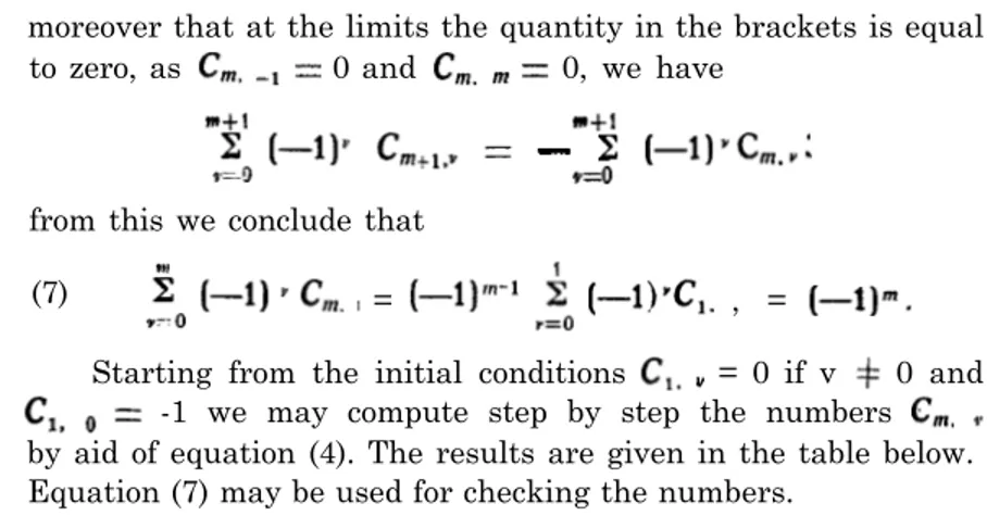
+ . . . + (-1)”

.

This formula becomes especially useful if f(x) is such a function that we have (x) since then we have

that is, the argument of is independent of This is often important.

Example. Let f(x) _I . As we shall see later, we have

10

The function expressed by differences. From the first it follows that

Executed on f(x) this gives

=

+

+

. . . +

+

.

The expressed by means. From the second relation we deduce that

(

The operation executed on f(x) gives

(x) (x) + (x)

+ . . + f(x) .

Means expressed by successive values of the function. The second relation gives

=

=

and therefore we have

=

+

+

. +

I .

Means expressed by differences. From we get

Hence

11

Expansion of a function by methods. have

We

since the operation performed on f(z) gives f(x) for if Tberefore this is the symbolical expression of Newton’s formula

f ( x )

Hitherto we have only defined operations combined by polynomial relations (except in the case of therefore the above demonstration assumes that is a positive integer.

But the significance of the operation is obvious for any value of indeed if we always have

= f ( x ) .

To prove that formula (1) holds too for any values of x it is necessary to show that the operation is identical with that corresponding to the series

. . . .

This is obviously impossible if the series

+

. . . . +

1 2

interpolation or summation formula does not depend on whether the function is a polynomial or not (except the remainder term)

If certain conditions are satisfied, the expansion of operation symbols into infinite series may be permitted even if the function to which the operations are applied, is not a polynomial when the corresponding series is convergent. cit.

To obtain Newton’s backward formula let us remark that 1 and start from

Expanding the denominator into an infinite series we get

According to what has been said, this formula is applicable, first if x is a positive integer, if f(x) is a polynomial, and in the general case if the series

=

+

+

(

(-3) + , . . .

is convergent, and f(x) satisfies certain conditions. An interesting particular case of (2) is obtained for

and if the operation is performed on f(x), we have

h

1 3

Expanding and dividing by we get

In the same manner we have, if f(x) is a polynomial or if it satisfies certain conditions:

that is

Expansion of an alternate function. A function

defined for x 0, 1, 2, 3, . . . is called an alternate function. Starting from the second formula we deduce

This formula may only he applied if x is a positive integer, since otherwise even in the case of polynomials it is divergent.

been mentioned that the Calculus of Finite Differen-ces deals also with functions of a continuous variable. In this case it is possible to both the derivatives and the differences and to establish relations between these quantities. Relation between differences and derivatives. If we write Taylor’s series in the following manner:

f (x-+-h) f(x) + (x) + (x) , . .

I Written symbolically it will be

and therefore

(3)

1 4

member into a series of powers of and multiply this series by itself, and apply Cauchy’s rule of multiplication we obtain A’; multiplying again we get and so on. We could express this way the m -th difference by derivatives, but we will obtain this later in a shorter way by aid of Stirling numbers 67).

Starting from 1 we could write formally

=

In this form the second member has no meaning, but expanding it into a power series it will acquire one:

+ . . . .

This formula gives the first derivative expressed by differences. It holds if the function is a polynomial, or if the series is convergent and satisfies certain conditions.

Again applying Cauchy’s rule we obtain then and so on. We could thus get the expression of the m -th derivative, but we shall determine it in another way 56).

7. Receding Differences. Some authors have introduced besides the differences considered in the preceding paragraph, called also advancing differences, others, the receding differen-ces. defined by

(x) f(x) f (x-h).

The symbol is that used by in our notation this will be

a n d =

Since the formulae containing symbols of receding dif-ferences are very easily expressed by formulae of advancing differences, and since there is no advantage whatever in introducing the receding differences, they are only

mentioned here.

cit. different notations have been proposed for the receding differences. Steffensen cit. 1, pp. 2241 puts

1 5

8. Central Differences. If we accept the notation of the advancing or that of the receding differences, there will always be a want of symmetry in the formulae obtained. Indeed, to have symmetrical formulae the argument of the difference

should be and therefore the difference corresponding to the argument x would be

f f

This has been adopted in the system called Central Differ-ences. Different notations have been proposed; we will adopt Sheppard’s notation, which is the following for the first central difference’

(x) f

and for the first Central Mean

= I .

From the above formulae it follows immediately that and (x) =

Moreover from these relations we easily deduce the following: (x) (x-nh)

(x) (x-nh)

=

( x ) = ( x - n h - h ) .

The connection between the formulae of the advancing and those of the central differences may be established easily by the calculus of symbols. Starting from

An excellent monograph on Central Differences is found in Sheppard cit. 3. Of the other notations let us mention [see

Robinson cit. 1. f(x)

The notation of the Central Mean introduced by Thiele and adopted by cit. 1. is the following

1 6

we obtain

and so on.

Working with central differences there is but one difficulty, since generally the function f(x) is given only for values such as f(x+nh) where n is a positive or negative integer. In such cases f or f has no meaning, nor have (x) and (x). But there is no difficulty in determining

(x), (x) and (x).

Returning to our table of differences 4) written in the advancing system, we find for instance the following line

( a ) . ,

If in this table we had used the central difference notation the numbers of the above line would have been denoted by

f

_{. .}

That is, the argument would have remained unchanged along the line. This is a simplification.

Since in the notation of central differences the odd ones are meaningless, the difference

must be expressed by aid of the even differences and by

To obtain an expression for we will start from the above symbolical expressions, writing

= + 2 M A = 2 A E

From this we get the important relations

A

Symbolical methods. We have seen in that

17

e _{2 sinh}

and

Starting

M

1

from these formulae we may determine any symbolical central difference expression in terms of the derivatives, for instance and others.

To obtain we use the expansion of (sinh into a power series. The simplest way of obtaining this series is to express first (sinh by a sum of Since

2 sinh x

we have

I

In the second member the terms correspon-ding to and combined give

+ so that we have

( - 1 ) ”

From this it follows that

sinh 0.

For we find

(2) sinh x) = 2 ( - 1 ) ”

therefore the required expansion will be

18

Finally putting x we have

=

Expansion of powers of the derivative-symbol

D

Futting again we have

first derivative will be

(n+l) (2 sinh (2 sinh

Using formula (2) we obtain the 2m -th derivative of this expression

and finally

(n+l) (-1) I’

+

9. Divided differences. So far we have supposed that the function f(x) is given for . . , x,, and that the interval

h

is independent of i. Now we deal with the general problem where the system of x,, . . . . , may be anything whatever.

By the first divided difference of denoted by (xi) the following quantity is understood:

f

I The second divided difference of is

19

and so on; the m -th divided difference is

Xi

From these equations we may deduce successively

= +

0

and so on. Putting (x-x,,) (x-x,) . . , . (x-x,,) we may give to the general term the following form

(1) + . . . . +

_.

The divided differences may also be given by Vandermonde’s determinant

1 m - l

1 _{. . .} m - l

. . , . , . , . .

. . .

1 2 . . .

. . . .

1 . . .

NOW

we shall deduce an expression by aid of the divided differences.

First multiplying (x,) by then by (x,) and so on: (x,) by and finally by

we obtain

20

In consequence of the relation

it follows that the coefficient of in the preceding equation is equal to one, since it can be shown that

(x,) =

so that the coefficient of is equal to -1. Moreover it can be demonstrated that

therefore for these values the term will vanish from the equation and we have

= + + +

This is the required expression of the function by aid of divided differences, Putting into this equation x instead of and adding the remainder, we obtain Newton’s expansion for functions given at unequal intervals

= + +

i-. i-. + (x-x,) (x-x,) . . .

We shall see in 123 that the remainder of the series is equal to

R

where is included in the interval of x, x,, , . , . Formula (3) may be written

+ +

21

Probability is that of the Generating Functions, found by and first published in his Analytique des

Paris

Given a function f(x) for . . b-l u(t) will be defined as the generating function of f(x) if the coefficient of in the expansion of u(t) is equal to f(x) in the interval a, and if moreover this coefficient is equal to zero for every other integer value of X. Therefore we have

u(f) f(x)

To denote that u(t) is the generating function of f(x) we shall write

=

If is infinite, the generating function of f(x) will be considered only for values of for which the series is convergent.

Remark. Another function may be determined so that the coefficient of shall be equal , in certain intervals, to the , function f(x) given above.

For instance, denoting by f,,,(x) the number of partitions of order m, of the number x (with repetition and permutation of 1, 2, n), it is easy to see that the generating function cf f,(x) is the following:

u(f) + , . , + f”)”

but for the expansion of the function

= . , ,

leads to the same coefficient as the function u(f). Since the expansion of u,(f) is simpler than that of u(f), we will use the former for the determination of f(x). We get

(f) =

Finally we have

22

To determine the generating functions there are several methods.

First method. In Infinitesimal Calculus a great number of expansions in power series are known. Each function expanded may be considered as a generating function. For instance we found:

Where the numbers are the Stirling Numbers of the first kind. We shall see them later

23

numbers are

Euler

numbers 105).

B

12. = =

The numbers are

Bernoulli

numbers 78)

Second method.

Starting from the generating functions obtained by the first method we may deduce, by derivation, integration, or other operations, new generating functions. Of course the conditions of convergence needed for these opera-tions must be fulfilled.

For instance starting from formula (1) we remark that the series is uniformly convergent for every value of such that 1. Therefore all derivative of the series, may be determined by term by term differentiation in the domain

I 1. The first derivation gives after multiplication by

13. so that = l

The -th derivative obtained from formula multiplied by gives

14.

I =

Formula (1) may also be integrated term by term and we get

15. =

if

In

this way we obtain again formula (3). A second integration will give

x ( x - 1 )

G

_{x ( x - 1 )} = ( l - 4 )

i f

Third method.

Sometimes it is possible to obtain the ge-nerating function of

f(x)

by performing directly the summation

2 4

First, this is possible if f(x) is &he x -th power of a number then we have

U ( t )

Example. Let f(x) cos cos is the real part of therefore a(t) will be the real part of

1

This is easily determined and we find

17. 1 cos

1 2t cos +

Secondly, the summation may be executed directly if it is possible to express the function f(x) by a definite integral in such a way that under the integral sign there figures the x power of some quantity independent of x. For instance if we have

then we shall have

In this manner we obtain in the form of a definite integral whose value may be known.

Example. Let f(x) We shall see later that the binomial coefficients are given by Cauchy’s _{formula 22.}

from this we conclude

25

tables of de we find that this integral is equal to

1 we may give the generating function this

simpler form

1

u ( f ) ₌

Remark 1. Since

2 ( $ 7 ; ‘ ) = 2

we have

2 x - l

Remark II. Starting from the above result we may obtain generating functions of many other expressions. For instance according to rule of multiplication of series we obtain from (18)

moreover

[ u ( f ) ] ’ 4”

Hence noting that the coefficients of are the same in the two expressions we get

This is a very useful formula.

11. General rules to determine generating functions.

1. The generating function of the sum of functions is equal to sum of the generating functions

[f,(x)

2 6

2. If c is a constant, then we have

Therefore, for instance, if a polynomial of degree is given by its Newton expansion

f ( x ) = f ( 0 ) (f) . . . .

then according to these rules we shall obtain the generating function of f(x) by aid of formula (14) of 10. We find

1

3. Given the generating function of f(x) f(x) u(t) f(x)

we may easily deduce the generating function of f indeed from the preceding equation we may obtain

u ( f ) - f ( O )

=

Therefore the generating of the of will be

- f ( o ) )

In the same manner we have

( 3 ) ---f(O) . .

The last formula us to the

tions of or of and so on, Example. We that

27

Determination of the generating function of t(x) starting from a difference equation. If the function f(x) is not directly given, but we know that it satisfies the following equation for x 0

+ f(x+n-1) . + a,,f(x) V(x) where the are independent of x and V(x) is a given function of x then we shall call the expression (4) “a complete linear dif-ference equation of order n with constant coefficients” If we denote the generating function of f(x) by u(t), the preceding rules (3) permit us to express the generating function of the first member of (4) by aid of u(t); if we know moreover the generating function R(t) of V(x), then, the generating functions of both members we obtain an ordinary equation of the first degree in u(t) solving this we have finally the generating function of f(x).

u ( t ) .

f .

Example. Let us suppose that the generating function of f(x) is required, and that f(x) satisfies the following equation for

0.

Therefore from (5) it follows that

(7) (0) log (l-t) _l--f

28

4. Starting from the generating function of f(x) we may obtain immediately the following generating functions

x ( x - 1 ) ( x - 2 ) , . . ( x - m + l ) f ( x )

and in the same manner as before

x(x-1) . . . ( x - m + l ) f =

u(f) -f(O) . . ( n - l )

1 .

Other simple particular cases are

=

=

a n d s o o n .

By aid of these formulae we may determine the generating function of f(x), if f(x) is given by a linear difference equation whose coefficients are polynomials of x.

We shall call the expression x(x-1) (x-2) . . , (x-m+l) ‘factorial of degree m’and denote it by (x),. If we expand the

coefficients of the difference equation into factorials, the equation may be written

=

By aid of the above relations we deduce from this equation a linear differential equation of which will determine the required generating function.

that is u(f). The solution of this differential equation is easily obtained by integration. We find

29

To determine the constant c let us remark that = f(0) therefore

12. Expansion of functions into power series. If func-tion f(x) is unknown but we have determined its generating function u(t), then to obtain f(x) we have to expand u(f) into a power series. In the Calculus of Finite Differences this occurs for instance when solving difference equations by the method of generating functions. In the Calculus of Probability very often it is much easier to determine the generating function of a quan-tity than the quanquan-tity itself. In these cases also we have to expand the obtained generating function.

The methods for expanding functions into power series are found in the treatises for Infinitesimal Calculus. Here only the most useful will be given.

method. Expansion by division. Example: 1

-

-l - f 1 f . . . . . .

Second method. Stirling’s of expansion of [Methodus Differentialis, 1730. 2). Let us put

1 _{f(0) f}

multiplying both members by the denominator. We must have

1 (0)

moreover the coefficient of must be equal to zero for every

o f T h i s gives 0 and the following

equation

(x-l) 0.

30

This method is known as that of indeterminate coef-ficients.

Third method. Expansion by the binomial theorem. Examples.

(3) .

= ,

Example 1.

and finally the coefficient of will he

= ( =

Example 2.

(5) , , . + (l-f)-”

(-1) ( .

To obtain the coefficient f(x) of we have to put (m+ l).We find

f ( x ) ( .

Example 3. Given Applying the bino-mial theorem we have

= .

I A second application of the theorem gives

.

Putting the coefficient f(x) of will be

(

31

Hence we have to for

successive differentiation, For instance if is equa to to sin etc.

factors p(f) , then we may apply

(7)

C. Derivation of unction of function. [See

Compendium II. us write u(y) and y We

have

d u _-du dy = d y

du

-

-d y

where the functions are of u. Therefore we may determine them by choosing e most convenient function ,

Let

Consequently

32

Moreover,

hence

from this it follows by aid of (7’) that

so that

Finally we have

For every particular function y we may determine once for the quantities , , , . , Y,,.

Example 1. Let y We may write

( )

hence

.

Putting h 0 and dividing by s! we get

( s - i ) “ .

We shall see in 58 that putting the second member will be equal to a Stirling number of the second kind.

SO

that

and

.

33

Example 2. Let y We shall have

moreover

Putting every term will vanish except that in which

Therefore we find

, =

Example 3. Let y We have

Proceeding in the same manner as in the preceding example we get

of a function of function by Faa Bruno’s formula.

Given and let us write

Y =

+

DY, + (x-x,)’

₊

₊

and

II 1

l

and secondly in consequence of the above equation to

,

, . . . ( , , .

so that finally we may write

,

a,. , . .

n ! . .

34

where

and .

a, + + . , . +

Remark. Comparing formulae (8) and (9) we find

=

_,

. , .

. , ,

n!

13. Expansion of functions by aid of decomposition into partial fractions. Let the following function be given

where and are polynomials; the degree of being less than that of We may always suppose that (t) and have no roots in common; since if they had, it would always be possible to simplify the fraction, dividing by f-r,,, , if i s

the root. .

35

Reducing the fractions to a common denominator we obtain u if for every value of we have

therefore this is an identity: so that the coefficients of in both members, must be equal, This gives equations of the first degree which determine the coefficients

But these may be determined in a shorter way. Indeed

= . , . .

therefore putting into the above equation every term will vanish except that of and we shall have

I

so that

and therefore

Finally the coefficient f(x) of in the expansion of u will be equal to

Example

Let

u(t)

2t

From this we deduce

= 5) and = Hence we have

= - 1 + a n d

Since it follows that

a n d

36

this gives

and finally

=

,

We could have obtained the same result by solving the difference equation deduced in Sfirling’s method (Method II,

12).

On the other hand the third method giving the expansion of the trinomial

would lead to

- 2

Putting x we obtain

f ( x ) = - 2

Equating this result to (1) gives the interesting relation

2. Decomposition of the reciprocal factorial

u(t) 1 (t-l) (t-2) . , . . (t-m),

m

1

. . .

therefore

37

1 . , .

B. The of are all single, but there are complex roots among The coefficients of y(t) are real: therefore if is a root of y(t) = 0,

will be a root too. The preceding method is still applicable but the corresponding values of a, ‘and a, will be complex conjugate:

Therefore the decomposition of u will be

This may be written

The expansion of the trinomial has been shown in Method III 12); putting into formula (6) -1, -2a and

we obtain

( 2 a )

This multiplied by the numerator gives

+ ,

- 2 ( 2 a )

,

Ch. 2. p. 261-266, Paris 1873.

38

Putting into the first expression and into the second we obtain finally

2

+

, , . .

C. The roots , . . . , of the polynomial are all real, but there are multiple roots. Let us suppose that the multiplicity of the root is where may be equal

1, 2, 3, . , and so on. The general formula of decomposition into partial fractions is the following:

If we multiply this expression by we get

= + . . . + ,

We have

. ,

Hence if we denote the first member of (4) by

A,.(t),

will be different from zero:

=

In the same manner the first derivatives give

This operation repeated for every value of v will give the required coefficients , Finally we shall have

This may be written

39

Therefore the coefficient f(x) of in the expansion of this expression will be

f(x) -‘A,

(m

D. Multiple complex roots. Let us suppose that the roots and are of the multiplicity m. We may write the fraction in the following manner

To obtain the coefficients and let us multiply this

equation by [ + denoting

A ( t ) we shall have

(5) A(t) +

-I-+ [(t-a) + . . . . , + From this we obtain immediately

= + +

We should have also

(7)

The last two equations-permit US determine and the second one superfluous; indeed knowing that a, and are real, by equating first the real parts in both members of and then the imaginary parts we get the two necessary equations.

The first derivative of A(t) for

=

+

+

This gives again two equations. Determining for

4 0

Example 3. Let We have

1

A(f) + +

+

Putting gives

Hence

A + +

+ 0 and 1 or

1

= ₄

The first derivative of A(f) gives for

=

=

+ .

From this it follows that

that is

a n d 1

1

= 16 a n d

To obtain c we multiply A(f) by (f-l) and put getting

If the coefficients and are calculated we may expand each term

+

using Method the expansion of a trinomial. Here we have

to put in formula (6) of 12 -2a and

41

other singularities in the interior or on the boundary of the circle of. radius then f(x), the coefficient of in the expansion of u(f), is given, according to a known theorem of by the following integral taken round this circle:

Putting and therefore dt we obtain

f ( x )

0

Example. Let (1 If is a positive integer then has no poles in the circle of unit radius. Putting we have

f ( x )

writing we obtain

+

0

I

cos cos a da.

Remarking that the coefficient of in the expansion of u(t) is equal, according to Newton’s rule, to , and moreover

0

that the above integral taken between the limits 0 and is equal to the half of that taken between the limits 0,

we conclude that

This is Cauchy’s formula expressing the binomial coefficient by a definite integral.

15. Expansion of a function by aid of difference equations.

42

u ( f ) R(f) . + + . . . +

+ + . , + +

then may be considered as being the generating function of a function f(x) determined by the difference equation

+ + , , . +

=

Indeed, we have seen (formula 5. 11) that the generating function of f(x) deduced by aid of the difference equation (2) is

(3)

f(i)

u ( f ) =

a,

where R(f) is the generating function of that is, V(x) is the coefficient of in the expansion of R(f).

Knowing V(x), let us suppose that we are able to solve the difference equation (2) by a method which does not require the expansion of the generating function (3). If we find f(x) = c,,) where the c are arbitrary constants, then we shall determine them by identification of (1) and and thus obtain the n equations:

(4) a ,

in the corresponding values of f(x) we may determine the n arbitrary constants a,,, , and obtain in this way the required coefficient f(x) of in the expansion of u(f).

Example 1. The function u(f) is to be expanded into a series of powers of According to what has been said, if we denote by f(x) the coefficient of in this ex-pansion then f(x) will be the solution of the difference equation

f (x+2) + 0.

We shall see in 165 that the solution of this equation is

43

From (4) we get

(0) or 0 f(0)

+ 1 = + f(1)

therefore

f(0) = 0 and f(l) 1.

these values into (5) we may determine the constants we find c, a n d Finally we have

If we do not know the solution of the difference equation (2) the method may still be applied. Starting from equation (4) we determine as before the values f (0), . . , , f (n-l) and then, by aid of equation (2) we compute step by step the values f(n), and so on.

E x a m p l e 2 . [ L e o n a r d o in Analysin Infinitorum 1748. Lausanne, 2 8 0 . The function u(t)

is to be expanded into a power series. The coefficient f(x) of is given by the difference equation:

0

Without solving this equation we get from (4)

+ or 1 = f(2)

= 0 = f(1)

(0) 0 f(0).

Hence

f(0) 0, f(1) 0, f(2) = 1.

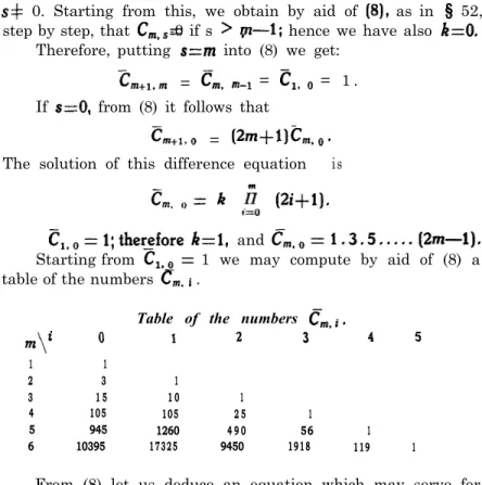
By the aid of these values we obtain from (6) step by step f(3) 6, f(4) f(5) f(6)

and so on.

R e m a r k . This method is identical with that of (Method II, 12). Given the function