Full Terms & Conditions of access and use can be found at
http://www.tandfonline.com/action/journalInformation?journalCode=ubes20
Download by: [Universitas Maritim Raja Ali Haji] Date: 11 January 2016, At: 22:37
Journal of Business & Economic Statistics
ISSN: 0735-0015 (Print) 1537-2707 (Online) Journal homepage: http://www.tandfonline.com/loi/ubes20
Flexible Bivariate Count Data Regression Models
Shiferaw Gurmu & John Elder
To cite this article: Shiferaw Gurmu & John Elder (2012) Flexible Bivariate Count Data Regression Models, Journal of Business & Economic Statistics, 30:2, 265-274, DOI: 10.1080/07350015.2011.638816
To link to this article: http://dx.doi.org/10.1080/07350015.2011.638816
View supplementary material
Accepted author version posted online: 20 Dec 2011.
Submit your article to this journal
Article views: 316
Supplementary materials for this article are available online. Please go tohttp://tandfonline.com/r/JBES
Flexible Bivariate Count Data Regression
Models
Shiferaw GURMU
Department of Economics, Andrew Young School of Policy Studies, P.O. Box 3992, Georgia State University, Atlanta, GA 30302 ([email protected])
John ELDER
Department of Finance & Real Estate, Colorado State University, Fort Collins, CO 80523 ([email protected])
The article develops a semiparametric estimation method for the bivariate count data regression model. We develop a series expansion approach in which dependence between count variables is introduced by means of stochastically related unobserved heterogeneity components, and in which, unlike existing commonly used models, positive as well as negative correlations are allowed. Extensions that accommodate excess zeros, censored data, and multivariate generalizations are also given. Monte Carlo experiments and an empirical application to tobacco use confirms that the model performs well relative to existing bivariate models, in terms of various statistical criteria and in capturing the range of correlation among dependent variables. This article has supplementary materials online.
KEY WORDS: Censoring; Multivariate counts; Negative correlation; Series estimation; Tobacco use; Unobserved heterogeneity.
1. INTRODUCTION
The main focus of this article is on series estimation of bivari-ate count data regression models with more flexible correlation structure. Multivariate count data regression models arise in sit-uations where several counts are correlated and joint estimation is required. For example, common measures of health care uti-lization, such as the number of doctor consultations, the number of other ambulatory visits, and prescription drug utilizations, are likely to be jointly dependent. Other leading examples in-clude the number of hospital admissions and the number of days spent in hospitals, the number of voluntary and involuntary job changes, the number of firms which enter and exit an industry, and the number of patents made and articles published by sci-entists (Mayer and Chappell1992; Cameron and Trivedi1993; Jung and Winkelmann 1993; Hellstrom 2006; Stephan et al.
2007). Gurmu and Trivedi (1994) and Cameron and Trivedi (1998) provide overviews of some of the earlier multivari-ate count data regression models. Kocherlakota and Kocher-lakota (1992) and Johnson, Kotz, and Balakrishnan (1997) discussed the statistical properties of multivariate discrete distributions.
Applications of these models in economics, statistics, and related fields have largely been confined to the bivariate Pois-son, bivariate negative binomial (NB), and bivariate Poisson-lognormal mixture regression models. The bivariate Poisson model imposes the restriction that the conditional mean of each count variable equals the conditional variance. This can result in misspecification of the marginals. For the common case of overdispersed counts, the bivariate (or multivariate) negative binomial model is potentially useful. However, the multivariate NB model imposes ad hoc conditions on the form of the distribu-tion of the common unobserved heterogeneity term affecting the counts. In estimation of truncated and censored models using a fully parametric approach, a misspecification of the distribution
of unobservables leads to inconsistency. Since the conditional means in these models depend on the density, the form of the density will affect the consistency of the regression parameters. A general flexible framework of estimation that does not require knowledge of the distribution of the unobservables is desirable. Existing commonly used bivariate count models have an-other potential shortcoming: they accommodate only nonneg-ative correlation between the counts. The statistics literature gives examples and general techniques on constructing nega-tively correlated multivariate Poisson distributions having Pois-son marginals; see, for example, Kocherlakota and Kocher-lakota (1992) for a review of this literature and Ophem (1999) for a related approach. In particular, Aitchison and Ho (1989) considered a multivariate lognormal mixture of independent Poisson distributions. Since the resulting mixture, the Poisson-lognormal distribution, does not have a closed form solution, estimation of the model requires numerical integration (Munkin and Trivedi1999; Hellstrom2006). The approach also requires knowledge of the distribution of unobserved heterogeneity com-ponents. From the practical point of view, it is desirable to have flexible methods that allow for both positive and negative corre-lations between the dependent variables. This article addresses these issues.
This article develops semiparametric (SP) methods for esti-mation of various mixture bivariate count models that allow for negative as well as positive correlations between the counts. In the context of models with two-factor unobserved heterogeneity components, this article employs a series expansion approach to model the joint distribution of unobserved heterogeneity com-ponents in the context of a bivariate Poisson mixture. To this
© 2012American Statistical Association Journal of Business & Economic Statistics April 2012, Vol. 30, No. 2 DOI:10.1080/07350015.2011.638816
265
end, we begin by analyzing the role played by the distribution of unobserved heterogeneity in the sign and magnitude of the correlation between counts. We also present methods for esti-mating truncated and censored bivariate regression models as well as extensions to zero-inflation and multivariate models. These extensions can be found in the online Supplemental Ap-pendix. Simulation experiments and an application to tobacco consumption are presented. The application involves joint mod-eling of the use of smoking tobacco and chewing tobacco as reported in a survey of households.
The general approach is a multivariate generalization of the semiparametric techniques developed for univariate count re-gression models (Gurmu 1997; Gurmu, Rilstone, and Stern
1999). Semiparametric estimators based on squared polyno-mial series expansions provide consistent estimates (Gallant and Nychka1987; Gurmu et al.1999; Bierens2008). As compared to flexible univariate methods, joint estimation of equations with correlated dependent count variables is expected to improve ef-ficiency. In principle, if interest is only on estimation of the pa-rameters of the conditional mean function in a multivariate count model, seemingly unrelated non-linear least squares estimation methods may be feasible, provided the underlying model allows for flexible variance and correlation structures. However, apart from estimation of parameters of economic interest, the focus of interest in most count regression models is consistent estimation of cell probabilities for different counts. The proposed series ex-pansion approach provides flexible specifications for the joint distribution of the counts as well as the marginals. In addition to estimating the expected number of counts and the correlation be-tween pairs of endogenous variables, the series method provides consistent estimates of joint probabilities of event counts, con-ditional on covariates. Correlations between jointly distributed variables are not restricted to be nonnegative. Further, methods based on first- and second-order moments alone are not directly applicable to truncated and censored models. The semiparamet-ric approach is particularly useful for truncated and censored regression models, where misspecification of the density leads to inconsistency. In a recent article, Gurmu and Elder (2007) analyzed a special case of the bivariate model proposed in this article based on first-order series expansion.
The remainder of the article is organized as follows. The next section develops a method for flexible series estimation of a bivariate mixture count data regression model. Section 3 eval-uates the feasibility and performance of the proposed method using Monte Carlo experiments. An application to individual tobacco consumption behavior is given in Section 4. Section 5 gives concluding remarks. Derivations of main results are given in Appendix A.1. Generalizations, detailed derivations, and fur-ther results from simulations and applications are provided in online Supplemental Appendices.
2. TWO-FACTOR BIVARIATE MODEL
2.1 The Framework
A major shortcoming of standard models such as the bivariate Poisson and bivariate NB models is that they do not allow for negative correlations between the count variables. This restric-tion arises from the assumprestric-tion of a common unobserved
het-erogeneity component used in the underlying mixing or convo-lution technique, resulting in the correlation between the counts being introduced through a dispersion parameter. We consider a two-factor framework in which dependence between count vari-ables is introduced through correlated unobserved heterogeneity components.
Consider two jointly distributed random variables,Y1andY2,
each denoting event counts. For observationi(i=1,2, . . . , N), we observe{yj i,xj i}2j=1, wherexj iis a (kj×1) vector of
covari-ates. Without loss of generality, the mean parameter associated withyj ican be parameterized as
θj i=exp(x′
j iβj), j =1,2, (1)
whereβjis a (kj ×1) vector of unknown parameters. We model
the dependence betweeny1andy2by means of correlated
unob-served heterogeneity componentsν1andν2. Each of the
compo-nents is associated with only one of the event counts. Accord-ingly, forj =1,2, suppose (yj i |xj i, νj i)∼Poisson (θj iνj i)
with (ν1i, ν2i) having a bivariate distributiong(ν1i, ν2i) inR2+.
Then the ensuing mixture density can be expressed as
f(y1i, y2i |xi)=
2
j=1
exp(−θj iνj i)
θj iνj i
yj i
Ŵ(yj i+1)
× g(ν1i, ν2i)dν1idν2i. (2)
LetM(−θ1i,−θ2i)=Eν[exp(−θ1iν1i−θ2iν2i)] denote the
bi-variate moment-generating function (MGF) of (ν1i, ν2i)
evalu-ated at (−θ1i,−θ2i). It can readily be seen that, analogous to the
one-factor error model (e.g., Gurmu and Elder2000), (2) takes the form
f(y1i, y2i|xi)=
2
j=1
θj i
yj i
Ŵ(yj i+1)
M(y1,y2)(
−θ1i,−θ2i), (3)
where, suppressingi,M(y1,y2)(−θ
1,−θ2)=∂y.M(−θ1,−θ2)/
(∂(−θ1)y1∂(−θ2)y2) is the derivative ofM(−θ1,−θ2) of order
y.=y1+y2.
The sign of the correlation coefficient between y1 and y2
is determined by the sign of the covariance between the two unobserved variables, cov(ν1, ν2). This is summarized in the
following proposition.
Proposition 1. In the mixture bivariate model (3), with the
assumption of independence betweenxandν, the covariance
between event counts takes the form
cov(y1i, y2i |xi)=θ1iθ2i[cov (ν1i, ν2i)].
where cov(ν1i, ν2i)=[M(1,1)(0,0)−M(1,0)(0,0)M(0,1)(0,0)].
Since θj i is nonnegative, sign (cov(y1i, y2i))=
sign(cov(ν1i, ν2i)).
The above result can be obtained using iterated expectations. The intuition about the sign of the correlation is as follows. In the case of univariate mixing, the correlation between the counts is affected only by the variance of the common unob-served heterogeneity term. Hence correlation is nonnegative. In the bivariate mixing, the variance of each unobserved compo-nents as well as the correlation between the compocompo-nents affect corr(y1i, y2i |xi). Hence, the sign of the correlation between
the count variables is determined by the allowed signs for the
Gurmu and Elder: Flexible Bivariate Count Data Regression Models 267
correlation between the unobserved heterogeneity terms, which generally may or may not be restricted.
Using the law of iterated expectations, the other low-order moments of the outcome variables, conditional on xi, can be
obtained as follows:
for any arbitrary mixing distribution forνi. While the sign of
the correlation between the event counts is unrestricted, the magnitudes of these correlations are narrower than the corre-sponding correlations from the mixing distribution. However, asθ1i andθ2i get larger, the gap between the two correlations
will be narrower, with corr(y1i, y2i |xi) getting very close to
corr(ν1i, ν2i). Aitchison and Ho (1989) derived similar bounds
for bivariate correlations between the count variables for mul-tivariate Poisson-lognormal mixture model without regressors. The correlation bounds in (7) apply to any arbitrary Poisson-unobserved factor mixture model, including the one proposed in this article.
The form of the density (3) depends upon the choice of the distribution of the unobservables,g(ν1i, ν2i). Ifg(.) follows a
bi-variate (or generally a multibi-variate) lognormal distribution, we get the bivariate (or multivariate) Poisson-lognormal distribu-tion proposed by Aitchison and Ho (1989). However, since the Poisson-lognormal mixture does not have a closed form, estima-tion of the unknown parameters requires numerical integraestima-tion. Nevertheless, the low-order moments, including correlations, of the multivariate Poisson-lognormal mixture distribution can easily be obtained (see Aitchison and Ho 1989). For exam-ple, Munkin and Trivedi (1999), Chib and Winkelmann (2001), and Hellstrom (2006) applied the Poisson-lognormal correlated model using simulated maximum likelihood (ML) or Markov chain Monte Carlo estimation methods.
We develop an estimation approach for model (3) that does not require knowledge of the distribution of the unobserved heterogeneity components. Another attractive feature of the approach is that, in addition to allowing for negative corre-lations, we obtain a closed form for the resulting correlated mixture model. The strategy is to approximate the density g(ν1i, ν2i) using techniques in bivariate density expansion. We
propose to take the approximate bivariate density to be of the general form
are orthonormal polynomials of degree k and r, respec-tively, defined on the respective marginal distributions;
and
is a constant of proportionality. The polynomial degreeK con-trols the extent to which the ensuing mixture modelf(y1i, y2i |
xi) deviates from the assumed baseline density. As discussed in
the following, whenK is set to zero in the proposed bivariate density ofy1andy2, we get a density that is a product of two
independent NB distributions. The polynomial degree param-eter is expected to increase with the sample size. In principle, the rule for increasing the size of series expansion can be data dependent (e.g., Gallant and Nychka1987). The parameterρkr
may be considered as the coefficient of correlation between the (k,r) polynomials in the bivariate distributiongN(ν1, ν2).
gN(ν1, ν2) are estimated within the likelihood framework. This
is discussed next.
2.2 Estimation
In our implementation, we use bivariate expansions based on generalized Laguerre polynomials. Let Lkj(νj i) denote the
relevantkth order generalized Laguerre polynomial associated with the random variableνj iwith baseline gamma weightw(νj i)
having parameters αj and λj, j =1,2; see Equations (A.1)
and (A.2) in Appendix A.1. The ensuingkth order orthonormal Laguerre polynomial takes the form Pk(νj i)=h−
Given the prevalence of gamma mixing in count and related duration models, the system of Laguerre polynomials is a natural choice.
The key result we need now is the approximate MGF, MN(−θ1i,−θ2i), and its derivative derived from the
approx-imate joint density based on Laguerre series expansion. The derivation of MN(−θ1i,−θ2i) is given in Appendix A.1. The
required derivative of this MGF is
M(y1, y2)
and
To construct the log-likelihood based on (3) and (10), we need to restrict the mean of each unobserved heterogeneity compo-nent to unity; that is, MN(1,0)(0,0)=1 and MN(0,1)(0,0)=1. As shown in Appendix A.1 [see Equations (A.6) and (A.7)], these conditions impose restrictions onλ1 andλ2. Hence, the
semiparametric (SP2) log-likelihood function based on bivariate mixing is
malization ρ00=1. SP2 denotes a bivariate semiparametric
model with two unobserved heterogeneity components. Like-wise, SPJ will denote a multivariate model withJunobserved heterogeneity components. SP will be used generically to denote the proposed semiparametric method for a class of multivariate count data models. As is conventional with orthogonal expan-sions (e.g., Lancaster 1969),P0(νj i)=1 andρ00 =1, so that
E[Pk(νj i)]=0 fork=1,2, . . . ,implying thatρkr =0 if either
korris zero, but not both. As explained in the paragraph follow-ing (8),ρkr =corr(Pk(ν1), Pr(ν2)) with respect to the
approx-imate bivariate distributiongN(ν1, ν2). For example, ifK=1,
the correlation parameter to be estimated is ρ11, where ρ11=
corr(P1(ν1), P1(ν2)) and P1(νj i)=(√αj−
in Equation (A.1) of Appendix A.1.
Due to the assumption of differential variances of the error components, the semiparametric approach provides a more flex-ible form for the variance of (yj i|xi) as compared to standard
one-factor bivariate count models based on mixing or convo-lutions. The correlation betweeny1 andy2 for anyKis given
in Appendix A.1, Equation (A.8). This correlation can take on zero, positive, or negative values. The correlation between the count series depends on the mean parameters (θ’s, henceβ’s), the dispersion parameters (α’s), and the correlation parameters (ρ’s). By contrast, if the unobservables logν1iand logν2iare
as-sumed to be distributed jointly as normally with mean vector 0, var(logνj i) = σj2, and corr(logν1i, logν2i) = τ, then corr(y1,
y2) implied by the ensuing bivariate Poisson-lognormal mixture
density depends onθ’s, theσ’s, and a single correlation param-eterτ. As discussed earlier following Equation (7), for both the Poisson-Laguerre Polynomial and Poisson-lognormal mixture models, the range of values taken by the correlation between y1andy2 is not as wide as that of the corresponding range of
correlation values betweenν1 andν2; they can be close when
θj’s are large.
The SP2 approach is based on the assumption of a baseline gamma density. Gamma mixing is a popular approach in appli-cations of count data and related models, including models of survival data. Since the SP2 density is based on gamma mixing, it nests the NB class of models. WhenK=0 (noteρ00=1),
we get a density that is a product of two independent NB distri-butions. IfK >0, we get a correlated bivariate density whose shape is modified by the presence of theρ’s and degree of series truncation. The bivariate count data model proposed by Gurmu and Elder (2007) is a special case of (13) withK=1. Anal-ogous to the Poisson–lognormal model, the SP2 density with K=1,may be thought of as a mixture of Poisson and bivari-ate gamma distributions. One of the main advantages of using the gamma baseline density is that it yields a computationally tractable closed form of the ensuing mixture model. As indi-cated by a referee, more polynomial terms (K) increase the set of possible distributional shapes obtained. One might argue that the correct choice of the baseline density is important for low
K, sayK=1. However, as explained below, this may not be an
issue if no specification error is detected for lowK.
The SP2 class of densities provides reasonable approxima-tions to count models that include densities with long upper tails, relatively skewed densities, and densities with low means as well as those with high means. The consistency of the pro-posed estimator can be shown using the framework developed by Gallant and Nychka (1987) and Gurmu et al. (1999). The pa-rameter space is a setB×M, whereβ∈B⊂RpandMis the
set of MGFs for positive random variables. Hereβ=(β′
1β2′)′.
Note that the estimators of the moment generation function are random sequence based on the approximating functiongN(.).
This requires thatK→ ∞asN → ∞, among other things. In general, the proposed series estimator may be considered as the quasi maximum likelihood estimator. Implementation of the estimator requires choosing the degree of the polynomialK. Following the literature on series estimation, one can use the Akaike Information Criterion (AIC) to chooseKor to compare different models. As argued by Gallant and Tauchen (1989), the truncated series expansion approach (K finite) may be viewed as finite-dimensional inference that has been subjected to a sen-sitivity analysis. That is, when specification error is detected, one increases the truncation pointK. In implementation, we use finite-dimensional inference (Kfixed) to compute standard er-rors. Comparison of bivariate models may also be based on how well they predict the cell probabilities,P(y1i =r,y2i =s), for
r, s=0,1,2, . . . .These issues will be considered further in the application section.
3. MONTE CARLO EXPERIMENTS
This section reports the results of Monte Carlo experiments that illustrate the feasibility and finite sample performance of the proposed estimation approach. The data-generating process (DGP) is based on the bivariate Poisson-lognormal mixture model, which is the basis of the estimation approach considered by Munkin and Trivedi (1999) and others. We also evaluate its performance relative to the bivariate NB maximum likelihood
Gurmu and Elder: Flexible Bivariate Count Data Regression Models 269
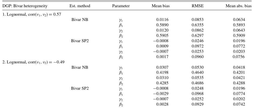
Table 1. Monte Carlo results on parameter estimates by bivariate count models
DGP: Bivar heterogeneity Est. method Parameter Mean bias RMSE Mean abs. bias
1. Lognormal, corr(ν1, ν2)=0.57
Bivar NB γ1 0.0116 0.0853 0.0634
β1 0.5890 0.6355 0.5893
γ2 0.0120 0.0862 0.0643
β2 0.5905 0.6297 0.5909
Bivar SP2 γ1 −0.0008 0.0246 0.0196
β1 0.0009 0.0972 0.0772
γ2 −0.0007 0.0253 0.0203
β2 0.0017 0.0960 0.0756
2. Lognormal, corr(ν1, ν2)= −0.49
Bivar NB γ1 0.0307 0.0530 0.0418
β1 0.4198 0.4640 0.4201
γ2 0.0310 0.0535 0.0421
β2 0.4285 0.4686 0.4288
Bivar SP2 γ1 −0.0008 0.0248 0.0196
β1 −0.0029 0.0968 0.0774
γ2 −0.0007 0.0252 0.0202
β2 0.0028 0.0929 0.0742
NOTE: The SP2 results are forK=2. The true values for the parameters areγ1=β1=γ2=β2=1.
estimator, which is commonly used in the applied literature due to its flexibility in handling overdispersed data.
We define an empirically relevant DGP with low means and overdispersed bivariate counts with varying assumptions about the distribution of unobserved heterogeneity, allowing for posi-tive as well as negaposi-tive correlations between the response vari-ables. Suppressing reference to observationi, the mean parame-ters of Poisson distributed count variablesy1andy2are specified
as
θj∗ =exp
γj+βjxj
νj, j =1,2. (14)
The values of explanatory variablesx1andx2are generated
in-dependently from normalN(0,1/16), with true values for the regression parameters set toγ1=β1=γ2=β2=1 in all
ex-periments. The unobserved heterogeneity termsν1 andν2 are
generated by bivariate uniform and bivariate lognormal distri-butions using the following specifications, along the implied average characteristics of the DGP.
(1) Bivariate lognormal with positive correlation: log(ν1)=ε1
and log(ν2)=ε2follow bivariate normal distribution with
mean (0,0), variancesσ2 1 =σ
2
2 =0.25 and correlation
pa-rameterρε=0.6. This gives mean(νj)=1.12, var(νj)=
0.37, and corr(ν1, ν2)=0.57 and average moments:
mean(yj)=3.08, var(yj)=8.40, and corr(y1, y2)=0.24.
(2) Bivariate lognormal with negative correlation: log(ν1)=
ε1 and log(ν2)=ε2 follow bivariate normal distribution
with mean (0,0), variances σ2
1 =σ22=0.25, and
cor-relation parameter ρε= −0.6. This implies mean(νj)=
1.12, var(νj)=0.37, and corr(ν1, ν2)= −0.49 and the
average moments: mean(yj)=3.08, var(yj)=8.40, and
corr(y1, y2)= −0.20.
(3) Bivariate uniform with correlation 0.6 with approximate moments: mean(νj)=1.0, var(νj)=0.33 and average
mo-ments mean(yj)=2.81, var(yj)=6.10, and corr(y1, y2)=
0.27.
(4) Bivariate uniform with correlation −0.6 with approxi-mate moments: mean(νj)=1.0, var(νj)=0.33 and
av-erage moments mean (yj)=2.81, var(yj)=6.10, and
corr(y1, y2)= −0.27.
Specifications 1 and 2 and the ensuing bivariate Poisson-lognormal mixture are based on the DGP used by Munkin and Trivedi (1999). Simulation experiments are based on sample size of 1000 with each experiment replicated 1000 times.
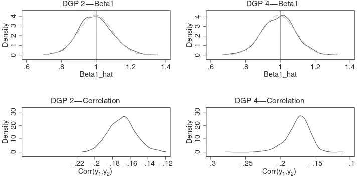
Table 1summarizes the simulation results in terms of mean bias, root mean squared error (RMSE), and mean absolute bias based on bivariate lognormal DGP.Figure 1gives kernel density estimates of the sampling distributions of ˆβ1(Beta1) and
corre-lations between the count variables from DGPs 2 and 4; model estimated by SP2 with K=2. Additional simulation results, including results using bivariate uniform DGP, kernel density estimates of the sampling distributions of coefficient estimates and estimated correlations, are given in the Supplemental Ap-pendix online. The results show that the SP2 estimates have low and insignificant biases under each of the 4 DGPs, irrespective of the values of the underlying correlations. The bias associated with any of the coefficients is less than 1% for SP2 withK=2. The RMSE is roughly about 2% for the intercept terms and about 10% for the slope coefficient estimates. Kernel density estimates demonstrate that, for a givenK, the sampling distributions of ˆγj
and ˆβj from SP2 are approximately normal. As expected, the
SP2 estimator performs much better than the commonly used bivariate NB estimator. Unlike simulation results for univariate NB of Gurmu et al. (1999), the biases associated with slope parameters resulting from bivariate NB can be quite substantial (35%–65%) even when data are uncensored. The variances of the slope estimates from bivariate NB associated with DGPs with negative correlations tend to be higher than those with positive correlations. The SP2 approach successfully predicts negative or positive correlations for all DGPs and even for each replication. However, the sampling distribution of the estimated
0
1
2
3
4
Density
.6 .8 1 1.2 1.4
Beta1_hat
DGP 2−Beta1
0
1
2
3
4
Density
.6 .8 1 1.2 1.4
Beta1_hat
DGP 4−Beta1
0
10
20
30
Density
−.22 −.2 −.18 −.16 −.14 −.12 Corr(y1,y2)
DGP 2−Correlation
0
10
20
30
Density
−.3 −.25 −.2 −.15 −.1 Corr(y1,y2)
DGP 4−Correlation
Figure 1. Kernel density estimates of distributions of coefficients and correlations DGPs 2 and 4, SP2 with K=2, sample size 1000. NOTE: The dashed lines in the top panel are the normal densities. For bottom panel, correlations were averaged over the sample observations prior to density estimation. The empirical average correlations between the count variables from DGPs 2 and 4 are−0.20 and−0.27, respectively.
correlations varies somewhat from the corresponding empirical distribution of correlations in all cases.
Using the bias-corrected simulated ML estimator with N =1000, 100 replications and 200 simulations, Munkin and Trivedi (1999; Table 1, page 41) reported mean estimates for parametersγ1, β1, γ2, andβ2in DGP 1 of 0.998, 1.012, 0.996,
and 1.009, respectively, with the corresponding standard er-rors of 0.028, 0.1, 0.028, and 0.097. By comparison, using the same design (DGP 1 with 100 replications), our SP2 param-eter estimates for γ1, β1, γ2, and β2 are 0.999, 0.997, 0.998,
and 1.014, respectively, with the corresponding standard de-viations of 0.028, 0.086, 0.029, and 0.110. The results for DGP 2 (lognormal heterogeneity with negative correlation) are qualitatively similar across both estimation methods; results for SP2 but based on 1000 replications are given in Table 1. Even though DGPs 1 and 2 based on lognormal heterogene-ity favor the Poisson-lognormal model employed by Munkin and Trivedi (1999), the proposed SP2 approach performs very well.
We use the means of the dependent count variables of between 2.8 and 3.1 in DGPs 1–4 to mimic reasonable applications of count data in the existing literature. We also carried out addi-tional simulations to explore examples of correlation bounds that might be encountered in practice. This is accomplished in two ways. First, we run two additional simulations to evaluate (a) the performance of the SP2 approach and (b) the bounds on the estimated correlation when the conditional means are very low—in the neighborhood of 0.7. Second, we calculate the correlation bounds from the two-factor bivariate mixture count models with varying heterogeneity assumptions and means of the counts, based on Proposition 1 and Equations (4)–(6). The means of the counts in this numerical exercise, which is not a Monte Carlo experiment, vary from 0.5 to about 40. This range captures most of the empirical applications.
The designs of the Monte Carlo simulation and calibration exercises as well as the results are provided in a Supplemental Appendix. The SP2 model again performs well in terms of bias and RMSE when the mean of the event counts is very low.
How-ever, as the mean becomes very small, the variance of the slope estimate tends to increase. The results also confirm that the mag-nitude of the correlation between the counts is narrower than the corresponding correlation from the distribution of unobserved heterogeneity components. As the means of the response vari-ables increase, the correlation between the counts approaches the correlation between the unobservables. On the other hand, as the means of the response variables decrease, the gap between the two correlations widens. This is potentially disconcerting since in many applications, the means of the response variables may be low. However, the proposed series expansion approach does a good job of estimating the magnitude and sign of the correlations from the underlying DGP. Next, we provide em-pirical applications involving event count variables with means ranging from as low as 0.3 to 3.2.
4. APPLICATION TO TOBACCO CONSUMPTION
As an example of an empirical application with negative cor-relation between counts, we consider an application to tobacco consumption behavior of individuals based on the 2001 house-hold Tobacco Prevalence Survey data from Bangladesh. The sur-vey was conducted in two administrative districts of paramount interest for tobacco production and consumption in the country. Data on daily consumption of smoking and chewing tobacco along with other socioeconomic and demographic characteris-tics were collected from respondents of 10 years of age and above. The dataset was used by Gurmu and Yunus (2008) in the context of binary response models. Here we focus on a 32% random sample consisting of 4800 individual respondents.
We consider joint modeling of two count variables: the daily number of smoking tobacco (Smoking) and number of chewing tobacco (Chewing). The average number of smoking tobacco used daily is about 3.2; the mean number of chewing tobacco is about 1.1 per day. The mean and standard deviations of both re-sponse variables show unconditional overdispersion. The range is 0–50 tobacco consumed per day for each of the counts. The count variables are unconditionally negatively correlated with
Gurmu and Elder: Flexible Bivariate Count Data Regression Models 271
a sample correlation of about−0.022, indicating that smoking and chewing tobacco may on average be substitutes. It is there-fore desirable to consider a joint modeling strategy that allows for both negative and positive correlations between the counts. The average respondent is a Muslim (78%), married (57%), in his/her early thirties, lives in a rural area, and has about seven years of formal schooling. Although the country is mostly agrar-ian, only around 11% of the respondents were related to agricul-tural occupation in either doing agriculagricul-tural operations on their own farms or working as agricultural wage laborers. About 12% of the respondents belong to the service occupation. The benchmark occupational group consists of business and other occupations. More than one-half of the fathers and slightly less than two-thirds of the mothers of the respondents currently use or have used tobacco products in the past. Detailed summary statistics are given in a Supplemental Appendix.
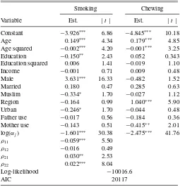
Table 2presents coefficient estimates from the proposed bi-variate count data model. Except forincomeand quadratics in
ageandeducation, the rest of the regressors are binary dummy
variables. The semiparametric model dominates the bivariate Poisson and bivariate NB models in terms of both the maxi-mized value of the log-likelihood function and the AIC. SP2 withK =2 yields the smallest AIC of 20,117 relative to AIC values of 48,061 and 28,776 for bivariate Poisson and bivariate NB models, respectively. The two-factor SP2 model also dom-inates the one-factor generalized bivariate NB model analyzed by Gurmu and Elder (2000) in terms of the AIC. Given the high proportion of reported zeros where about 65% of respondents are non-users of tobacco, we also estimate a zero-inflated (ZI) version of the proposed SP2 model withK=1 (AIC = 19,501). The estimates of the correlation parameters (ρ’s) associated
Table 2. Semiparametric coefficient estimates andt-ratios for smoking and chewing tobacco (SP2 withK=2)
Smoking Chewing
Variable Est. |t| Est. |t|
Constant −3.926∗∗∗ 6.86 −4.845∗∗∗ 10.18
Age 0.149∗∗∗ 4.34 0.179∗∗∗ 4.85
Age squared −0.002∗∗∗ 4.20 −0.001∗∗∗ 3.25
Education −0.150∗∗ 2.43 0.052 0.343
Education squared 0.006 1.41 −0.019 1.10
Income −0.001 0.71 0.009 0.48
Male 3.631∗∗∗ 16.33 −0.482 1.52
Married 0.180 0.47 0.285 0.63
Muslim −0.334∗ 1.70 −0.027 1.12
Region −0.164 0.99 1.040∗∗∗ 5.90
Urban −0.246∗ 1.70 −0.044 0.48
Father use −0.017 0.56 −0.184 0.36
Mother use −0.143 0.51 −0.415∗∗ 2.01
log(αj) −1.601∗∗∗ 30.38 −2.475∗∗∗ 41.76
ρ11 −0.059∗∗∗ 5.50
ρ12 −0.016 0.49
ρ21 0.030∗∗ 2.53
ρ22 0.022∗∗∗ 8.04
Log-likelihood −10016.6
AIC 20117
NOTE:∗∗∗, significant at 1%;∗∗, significant at 5%;∗, significant at 10%. Regression includes occupation effects.
with SP2 models show that modeling higher order polynomials of unobserved heterogeneity components is important.
The bivariate Poisson model seems to be inadequate for joint estimation of overdispersed count data. There are some differ-ences in the results from the semiparametric and the bivariate NB models. In particular, there are differences in the statistical significance of some variables such as occupational and regional dummy variables in both equations. Tobacco consumption is concave in age; tobacco smoking for example reaches a maxi-mum at about age 50. Male respondents consume significantly more smoking tobacco than women, while women tend to con-sume more chewing tobacco, a result which is in line with the custom of the country (Gurmu and Yunus2008).
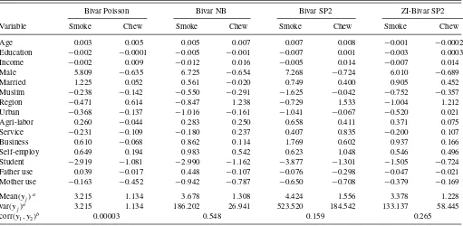
We also computed the average marginal effects of changes in the regressors on the mean number of daily tobacco use. The marginal effects from bivariate SP2, ZI bivariate SP2, bivariate Poisson, and bivariate NB are shown inTable 3. Generally the marginal effects from SP2 models are larger than those from the other bivariate models. The difference in the mean effects for various models is likely to be particularly important for sig-nificant regressors. The results from bivariate SP2 show that on average two additional years of schooling would reduce smok-ing by about a half stick of cigarette per month. On average, men smoke about seven cigarettes per day more than women.
The average of the correlations betweenSmokingand Chew-ingis about 0.55 for the bivariate NB model, 0.16 for Bivari-ate SP2, and 0.27 for ZI-bivariBivari-ate SP2. Given the characteris-tics of the individuals, the correlation between the two tobacco consumption variables estimated from ZI-bivariate SP2 model varies between a minimum of about−0.003 and maximum of 0.932 with 16.2% of the 4800 observations having negative correlations. These results suggest that, smoking and chewing tobacco may be substitutes for some individuals, rather than being complements for everyone.
Compared with univariate and bivariate standard models, there is preponderance of statistical evidence (e.g., using AIC and tests of independence) in favor of the SP class of models of tobacco use. Direct comparisons of the unconditional sample moments and estimated conditional and average (unconditional) moments are generally difficult because of the role of explana-tory variables and the sampling distributions of the estimated moments in the latter. For example, introduction of covariates will generally dampen the amount of conditional overdisper-sion. Subject to these caveats, comparisons of models show that the estimated average means, degree of overdispersion, and cor-relations from the SP2 model are generally consistent with the corresponding unconditional sample moments. The SP2 model fits the empirical distribution better than bivariate Poisson and NB models.
In an earlier version of this article, we provide an application to health care utilization measures, also given in the Supplemen-tal Appendix. Though not overwhelming, there are some differ-ences between the SP2 model and existing realistic competitors in the significance of the variables and estimated marginal ef-fects in both applications. Univariate models, such as NB model, that appropriately handle overdispersion are better than bivari-ate Poisson model. The usefulness of the bivaribivari-ate NB model in empirical applications is limited since it imposes correlation between series to be nonnegative. In general, the analysis in this
Table 3. Average marginal effects and average of moments of the number of daily tobacco use
Bivar Poisson Bivar NB Bivar SP2 ZI-Bivar SP2
Variable Smoke Chew Smoke Chew Smoke Chew Smoke Chew
Age 0.003 0.005 0.005 0.007 0.007 0.008 −0.001 −0.0002
Education −0.002 −0.0001 −0.005 −0.001 −0.007 0.001 −0.003 0.0003
Income −0.002 0.009 −0.012 0.016 −0.005 0.014 −0.007 0.014
Male 5.809 −0.635 6.725 −0.654 7.268 −0.724 6.010 −0.689
Married 1.225 0.052 0.561 −0.020 0.749 0.400 0.905 0.452
Muslim −0.238 −0.142 −0.550 −0.291 −1.625 −0.042 −0.752 −0.357
Region −0.471 0.614 −0.847 1.238 −0.729 1.533 −1.004 1.212
Urban −0.368 −0.137 −1.016 −0.161 −1.041 −0.067 −0.520 0.021
Agri-labor 0.260 −0.044 0.283 0.250 0.658 0.411 0.371 0.075
Service −0.231 −0.109 −0.180 0.237 0.407 0.835 −0.200 0.107
Business 0.610 −0.068 0.862 0.114 1.769 0.602 0.937 0.166
Self-employ 0.649 0.194 0.983 0.542 0.623 1.048 0.546 0.496
Student −2.919 −1.081 −2.990 −1.162 −3.877 −1.301 −1.505 −0.724
Father use 0.039 −0.017 0.448 −0.107 −0.076 −0.298 −0.047 −0.021
Mother use −0.163 −0.452 −0.942 −0.787 −0.650 −0.708 −0.379 −0.169
Mean(yj)a 3.215 1.134 3.678 1.308 4.424 1.556 3.378 1.228
var(yj)a 3.215 1.134 186.202 26.941 523.520 184.542 133.137 58.445
corr(y1, y2)b 0.00003 0.548 0.159 0.265
aSample averages of fitted marginal moments of smoking and chewing tobacco.bSample average of fitted correlations between smoking and chewing tobacco. The range of estimated correlation from ZI-Bivar SP2 model is−0.003 to 0.932.
article suggests that bivariate mixture models with a common unobserved heterogeneity component are inadequate in empir-ical applications, in that a single unobserved variable may not be able to account both for the dependence between the counts and for the variation in the dependent variables due to changes in unobservables.
To obtain satisfactory starting values for the mean parameters in both applications, we sequentially estimate standard bivariate count models, such as the bivariate Poisson and bivariate NB models. Using estimates from these models as our starting val-ues, the optimization algorithm for our model is typically able to achieve the usual gradient-based convergence criteria, resulting in substantial improvements in the log-likelihood function and AIC. As we increase the degree of polynomial, we use start-ing values from lower order polynomial model. At each step, we reinitiate the optimization procedure using different start-ing values to start a fresh search for a global maximum. In the Monte Carlo analysis, for small proportion of the replications, the optimization routine was restarted with slightly altered start-ing values. Although optimization algorithms cannot guarantee that they achieve the global optimum, we feel confident that our parameter estimates are valid given the plausibility and the qualitative aspects of our results.
5. CONCLUSION
This article has developed a flexible two-factor bivariate count data regression model based on series expansion for the joint density of the unobserved heterogeneity components. Multi-variate generalizations as well as extensions to accommodate truncated, censored, and ZI correlated count data models are provided. We obtain a computationally tractable closed form of
the bivariate model that allows for both negative and positive correlations. Our empirical application and simulation experi-ments show that the proposed model fits various features of the data well and compares favorably with existing bivariate count data models.
The gain in the proposed SP2 model comes from suitably modeling overdispersion as well as correlation between vari-ables within a flexible likelihood framework. As compared to the Poisson-lognormal mixture model, the SP2 model relies less on distributional assumptions and provides a closed form of the likelihood function. Note that the dispersion (α’s) and correla-tion (ρ’s) parameters also appear in the marginal distributions implied by the correlated SP2 model. When a test of the null hypothesis of independence is rejected, the SP2 model is ex-pected to fit both the bivariate distribution as well as the implied marginals better. If the correlation betweeny1andy2is not
sig-nificantly different from zero, the SP2 model is simply fitting the marginals better. However, if the test of independence is not rejected, it is more sensible to estimate flexible univariate mod-els such as those considered by Cameron and Johansson (1997), Gurmu (1997), and Gurmu et al. (1999).
As in univariate models, the semiparametric approach for multivariate models is particularly attractive for censored, trun-cated, and related modified models where parametric maximum likelihood estimates are not robust to misspecification of the error distribution. Monte Carlo results reported by Gurmu et al. (1999) show that biases and the sampling variances resulting from censored and truncated parametric models, such as the censored NB, can be substantial. Their Monte Carlo results from the regular (uncensored) sample show that although the SP procedure has an edge over standard parametric models, the biases resulting from parametric and SP models with hetero-geneity are not substantial. By contrast, the Monte Carlo results
Gurmu and Elder: Flexible Bivariate Count Data Regression Models 273
in this article show that the biases and sampling variances from the standard (uncensored/untruncated) bivariate models (such as bivariate NB model) may be substantial.
While the sign of the correlation between counts is un-restricted, the range of possible values from the Poisson-unobserved factor mixture models is generally narrower than that of the corresponding mixing distribution. The range of pos-sible correlations can be quite high in absolute terms for large values of the means of the counts, but this is not attainable in some common applications with small means. An ideal exten-sion of the method proposed in this article is to have a multi-variate generalization that achieves the full range of correlations between the counts.
APPENDIX: DERIVATIONS AND GENERALIZATIONS
A.1. Derivations and Some Expressions of the SP2 Model
We outline the derivation of the MGF based Laguerre series expansion. The relevantkth order generalized Laguerre polyno-mial associated with the random variableνj iis
Lkj(νj i)=
the constant of proportionality in Equation (9) takes the form
̟ =
the last two lines follow from the properties that E[Pk(νj)Pl(νj)]=0 fork =lby orthogonality of polynomials
and each with unit variance (E[Pk2(νj)]=1). The approximate
density will then take the form
gN(ν1i, ν2i)=
The main result we need is the MGF
MN(−θ1i,−θ2i)= exp(−θ1iν1i−θ2iν2i)gN(ν1i, ν2i) dν1idν2i,
wheregN(.) is given in (A.3). Using properties of orthonormal
polynomials and since the integration and expectations are taken with respect to the baseline marginal distributions, this MGF can be reorganized and expressed readily as
MN(−θ1i,−θ2i)=
We exploit the properties of the gamma function, Ŵ(γ)=
zγ−1e−zdz, and a two-parameter gamma density,
zγ−1e−z/δdz
=Ŵ(γ)γδ, to obtain a closed form solution for
this MGF. The approximate MGF corresponding to the ith observation is
Detailed derivations for (A.5) are available in the online Sup-plemental Appendix.
Next, we show the implications of restricting the mean of each unobserved heterogeneity component to unity. Using (10), set
MN(1,0)(0,0)=1 andMN(0,1)(0,0)=1. These restrictions yield
nally, the correlation coefficient for the SP2 model is
corr (y1i, y2i |xi)
This is obtained readily using the general results in Proposition 1 and Equation (7) with the mean of each unobserved hetero-geneity component set to unity.
Multivariate generalizations as well as extensions to accom-modate truncated, censored, and ZI correlated count data mod-els are provided in Supplementary Appendix B. Shaw (1988), Grogger and Carson (1991), Silva (1997), and Gurmu et al. (1999) provide background and applications of truncated and censored univariate count data models. See, for example, Wang (2003) and Gurmu and Elder (2008) for background, applica-tions, and recent developments in univariate ZI models.
SUPPLEMENTAL MATERIAL
Supplemental appendices B–G contain generalizations, ad-ditional derivations, results, tables, and graphs for the applications and Monte Carlo experiments. These ap-pendices and the GAUSS program used in this article can also be downloaded from the authors’ homepages (http://www2.gsu.edu/˜ecosgg/research/pdf/ge_jbes.pdf).
ACKNOWLEDGMENTS
The authors thank the co-editor, Keisuke Hirano, the asso-ciate editor, two anonymous referees, and numerous seminar and conference participants for helpful comments and sugges-tions. Mohammad Yunus graciously provided the data used in this article. Any errors that remain are solely our responsibility.
[Received September 2009. Revised August 2011.]
REFERENCES
Aitchison, J., and Ho, C. H. (1989), “The Multivariate Poisson-log Normal Distribution,”Biometrika, 76, 643–653. [265,267]
Bierens, H. (2008), “Semi-Nonparametric Interval-Censored Mixed Propor-tional Hazard Models: Identification and Consistency Results,”Econometric Theory, 24, 749–794. [266]
Cameron, C., and Johansson, P. (1997), “Count Data Regressions Using Series Expansions: With Applications,”Journal of Applied Econometrics, 12, 203– 223. [272]
Cameron, C., and Trivedi, P. K. (1993), “Tests of Independence in Paramet-ric Models With Applications and Illustrations,”Journal of Business and Economic Statistics, 11, 29–43. [265]
——— (1998),Regression Analysis of Count Data, Cambridge, UK: Cambridge University Press. [265]
Chib, S., and Winkelmann, R. (2001), “Markov Chain Monte Carlo Analysis of Correlated Count Data,”Journal of Business and Economic Statistics, 19, 428–435. [267]
Gallant, A. R., and Nychka, W. (1987), “Semi-Nonparametric Maximum Like-lihood Estimation,”Econometrica, 55, 363–390. [266,267,268]
Gallant, A. R., and Tauchen, G. (1989), “Seminonparametric Estimation of Conditionally Constrained Heterogeneous Processes: Asset Pricing Appli-cations,”Econometrica, 57, 1091–1120. [268]
Grogger, J., and Carson, J. (1991), “Models for Truncated Counts,”Journal of Applied Econometrics, 6, 225–238. [274]
Gurmu, S. (1997), “Semi-Parametric Estimation of Hurdle Regression Models With an Application to Medicaid Utilization,”Journal of Applied Econo-metrics, 12, 225–242. [266,272]
Gurmu, S., and Elder, J. (2000), “Generalized Bivariate Count Data Regression Models,”Economics Letters, 68, 31–36. [266,271]
——— (2007), “A Simple Bivariate Count Data Regression Model,”Economics Bulletin, 3(11), 1–10. [266,268]
——— (2008), “A Bivariate Zero-Inflated Count Data Regression Model With Unrestricted Correlation,” Economics Letters, 100, 245– 248. [274]
Gurmu, S., Rilstone, P., and Stern, S. (1999), “Semiparametric Estimation of Count Regression Models,”Journal of Econometrics, 88, 123–150. [266,268,269,272,274]
Gurmu, S., and Trivedi, P. K. (1994), “Recent Developments in Event Count Models: A Survey,” Thomas Jefferson Center Discussion Paper #261, De-partment of Economics, University of Virginia. [265]
Gurmu, S., and Yunus, M. (2008), “Tobacco Chewing, Smoking and Health Knowledge: Evidence From Bangladesh,”Economics Bulletin, 9(10), 1–9. [270,271]
Hellstrom, J. (2006), “A Bivariate Count Data Model for Household Tourism Demand,”Journal of Applied Econometrics, 21, 213–226. [265,267] Johnson, N. L., Kotz, S., and Balakrishnan, N. (1997),Discrete Multivariate
Distribution, New York: Wiley. [265]
Jung, R. C., and Winkelmann, R. (1993), “Two Aspects of Labor Mobility: A Bivariate Poisson Regression Approach,”Empirical Economics, 18, 543– 556. [265]
Kocherlakota, S., and Kocherlakota, K. (1992),Discrete Distributions, New York: Marcel Dekker. [265]
Lancaster, H. O. (1969),The Chi-Squared Distribution, New York: Wiley. [268] Mayer, W. J., and Chappell, W. F. (1992), “Determinants of Entry and Exit: An Application of the Compounded Poisson Distribution to US Industries, 1972–1977,” Southern Economic Journal, 58, 770– 778. [265]
Munkin, M., and Trivedi, P. K. (1999), “Simulated Maximum Likelihood Es-timation of Multivariate Mixed-Poisson Regression Models, With Applica-tion,”Econometric Journal, 1, 1–20. [265,267,268,269,270]
Ophem, H. van. (1999), “A General Method to Estimate Correlated Discrete Random Variables,”Econometric Theory, 15, 228–237. [265]
Shaw, D. (1988), “On-site Samples’ Regression: Problems of Non-Negative In-tegers, Truncation and Endogenous Stratification,”Journal of Econometrics, 37, 211–233. [274]
Silva, J. M. C. (1997), “Unobservables in Count Data Models for On-Site Samples,”Economics Letters, 54, 217–220. [274]
Stephan, P. E., Gurmu, S., Sumell, A. J., and Black, G. C. (2007), “Who’s Patenting in the University? Evidence From the Survey of Doctor-ate Recipients,” Economics of Innovation and New Technology, 16,71– 99. [265]
Wang, P. (2003), “A Bivariate Zero-Inflated Negative Binomial Regression Model for Count Data With Excess Zeros,”Economics Letters, 78, 373– 378. [274]