www.elsevier.com/locate/spa
Fluctuation of the transition density for Brownian motion
on random recursive Sierpinski gaskets
(B.M. Hambly
a;∗, Takashi Kumagai
baDepartment of Mathematics, University of Bristol, University Walk, Bristol, BS8 1TW, UK bGraduate School of Informatics, Kyoto University, Kyoto 606-8501, Japan
Received 18 April 2000; received in revised form 2 August 2000; accepted 3 August 2000
Abstract
We consider a class of random recursive Sierpinski gaskets and examine the short-time asymp-totics of the on-diagonal transition density for a natural Brownian motion. In contrast to the case of divergence form operators inRn or regular fractals we show that there are unbounded uc-tuations in the leading order term. Using the resolvent density we are able to explicitly describe the uctuations in time at typical points in the fractal and, by considering the supremum and inmum of the on-diagonal transition density over all points in the fractal, we can also describe the uctuations in space. c2001 Elsevier Science B.V. All rights reserved.
MSC:primary 60J60; secondary 60J25; 60J65
Keywords:Heat kernel; Laplace operator; Resolvent density; General branching process; Random recursive fractals
1. Introduction
The fundamental work of Aronson (1967), established upper and lower estimates on the heat kernel for an elliptic operator in Rn. There is now a substantial literature on the behaviour of the heat kernel for elliptic operators on manifolds, and that of the transition kernel for random walks on groups or graphs (see for instance Coulhon and Grigoryan, 1998; Davies, 1991). There are two components to the estimate, an on diagonal term, which is usually determined by the volume growth of the space, and the o diagonal term, where there is Gaussian decay.
The study of fractals has shown that the behaviour may be dierent when the geometry is not smooth. We state here the results for regular fractals F such as the Sierpinski gasket or the Sierpinski carpet. Ifpt(x; y) denotes the transition density for the natural Brownian motion on the fractalF (or the heat kernel for the corresponding
(Research partly supported by a Royal Society Industry Fellowship at BRIMS, Hewlett-Packard and
Grant-in-Aid for Scientic Research (B)(2) 10440029. ∗Corresponding author.
E-mail addresses:[email protected] (B.M. Hambly), [email protected] (T. Kumagai). 0304-4149/01/$ - see front matter c 2001 Elsevier Science B.V. All rights reserved.
Laplace operator on F), then there exist constants c1:1; c1:2 such that
pt(x; y)6c1:1t−ds=2exp −c1:2
d(x; y)dw t
1=(dw−1)!
; ∀x; y∈F; 0¡ t ¡1:
(1.1)
The exponent ds is called the spectral dimension and governs the asymptotics of the
spectral counting function, dw is called the walk dimension and is determined by the
time to distance scaling in the fractal, and d(·;·) is an intrinsic shortest path metric (in the case of Sierpinski carpet or gasket it is equivalent to the Euclidean distance). There is a corresponding lower bound of the same form but dierent constants. Note that if ds=n and dw= 2 we recover the usual Gaussian bounds of Rn. We will call
such upper and lower bounds Aronson-type estimates on the transition density (or heat kernel). For a discussion of these estimates and background results concerning diusion on fractals see Barlow (1998).
We will be interested in the situation where the geometry of the fractal is generated in a random way, and to determine the eect this has on the on-diagonal transition density. In a previous paper (Hambly, 1997), a natural Brownian motion on a random recursive Sierpinski gasket was constructed and relatively crude estimates obtained on its transition density. The estimates were not tight and indicated that it might not be possible to obtain the uniform Aronson type estimates of (1.1) in this setting.
One situation where fractals with irregular geometry were analysed in detail is the case of scale irregular fractals, discussed in Barlow and Hambly (1997) and Hambly et al. (2000b). These fractals are spatially homogeneous but not scale invariant with the irregularity given by an environment sequence. It is known that there is typically uctuation in the short-time asymptotics of the heat kernel and, in the Sierpinski gasket case, if the environment is generated by an iid sequence, an explicit description of the uctuation can be established. Using the relationship between the spectral counting function and the trace of the heat semigroup it can be shown that the spectral counting function also exhibits uctuation in its asymptotics.
The spectral counting function for random recursive Sierpinski gaskets was the sub-ject of Hambly (2000). It was shown that if N() denotes the number of eigenvalues of the Laplacian (Dirichlet or Neumann), then under a certain non-lattice assumption, there exists a non-zero mean one random variable W, and a constant c1:3 such that
lim
→∞ N()
ds=2 =c1:3W
1−ds=2; P-a:s:
This raises the question of whether there really are uctuations in the short-time asymp-totics of the heat kernel. In this paper we will show that there are uctuations and we identify their functional form (which is determined by the tails of the random vari-ableW). As the spectral counting function can be recovered from the trace of the heat semigroup, this shows that integrating over the fractal leads to the cancellation of these uctuations.
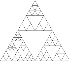
Fig. 1. A graph approximation to a random recursive Sierpinski gasket.
is a triangular fractal with generator consisting of 6 upward pointing triangles and 3 downward ones which are removed, for denitions see Hambly (2000)) we describe explicitly the uctuations in time and space. Let (;F;P) denote the probability space
of random recursive fractals F(!) built from the two fractals as in Hambly (1997) (a realization is shown in Fig. 1), where we choose type SG(2) with probabilitypand SG(3) with probability 1−p. The spectral dimension for the random fractal is given by ds=2 ==(+ 1), almost surely, where
:={s:p3(3=5)s+ (1−p) 6 (7=15)s= 1}:
Note that if we dene2= log 3=log(5=3) and3= log 6=log(15=7) the spectral
dimen-sion of SG(2) is given by 2=(2+ 1) = 2 log 3=log 5 and for SG(3) is 3=(3+ 1) =
2 log 6=log(90=7). We also need two correction exponents,′==
2−1; = 1−=3.
The Laplace operator is dened with respect to a measure induced by a suitable general branching process. This measure is equivalent to the Hausdor measure in the resistance metric (see Sections 3 and 4 for details).
Theorem 1.1. (1) There exists a jointly continuous transition density pt(x; y) for
x; y∈F and t ¿0.
(2) There exist constantsc1:4; c1:5 such that
c1:46lim sup
t→0
pt(x; x)
t−=(+1)(log|logt|)=(+1)6c1:5; -a:e: x∈F; P-a:s:
(3) There exist constantsc1:6; c1:7 such that
c1:66lim
t→0supx∈F
pt(x; x)
t−=(+1)(|logt|)=(+1)6c1:7; P-a:s:
(4) There exists a constant c1:8 such that
lim inf
t→0
pt(x; x)
t−=(+1)(log|logt|)′=(+1)6c1:8; -a:e: x∈F; P-a:s:
(5) There exists a constant c1:9 such that
lim
t→0xinf∈F
pt(x; x)
It is possible to obtain lower bounds in cases (4) and (5) but, though they have the same number of logarithms, we require a further assumption on the class of fractals and the exponent in the logarithmic terms diers.
This result is quite dierent to that for elliptic operators in divergence form on a bounded domain D⊂Rn, where
c1:126lim
t→0
pt(x; x)
tn=2 6c1:13; ∀x∈D:
In the case of regular fractalsF such as nested fractals (LindstrHm, 1990), or Sierpinski
carpets we have
c1:106lim
t→0
pt(x; x)
tds=2 6c1:11; ∀x∈F:
In these settings any uctuations for the leading order term in the transition density must be bounded.
We note here that extending these uctuation results to a wider class of random fractals, such as random recursive nested fractals not based ond-dimensional tetrahedra, is a non-trivial problem. The main diculty lies in establishing the existence of a Brownian motion on such fractals. It can be shown that there is no uniform Harnack inequality in that setting and hence the existence of the process is a serious diculty. The outline of the paper is as follows. In Sections 2 and 3 we introduce the random recursive Sierpinski gaskets and give a description of these sets via general branching processes. In Section 4 we introduce the natural Laplace operator on these fractals via its Dirichlet form and a natural measure. We also derive the crucial properties of these quantities. In Section 5 we show uctuations in the limiting random variable of the general branching process. Section 6 will show the uctuation in the on-diagonal transition density via a corresponding uctuation in the Green density. Throughout the paper we will label theith xed constant in Section n by cn:i, other constants ci may
be used in dierent proofs but will be xed within a given proof.
2. Random recursive Sierpinski gaskets
We construct our random recursive fractals from the class of ane nested Sierpinski gaskets and begin by recalling the denitions of such fractals (Fitzsimmons et al., 1994; LindstrHm, 1990). For l ¿1, an l-similitude is a map :Rd→Rd such that
(x) =l−1U(x) +x0; (2.1)
whereU is a unitary, linear map andx0∈Rd. Let ={ 1; : : : ; m} be a nite family
of maps where i is an li-similitude. For B⊂Rd, dene
(B) =
m [
i=1
i(B);
and let
n(B) = ◦ · · · ◦ (B):
As each i is a contraction, it has a unique xed point. Let F0′ be the set of xed
points of the mappings i, 16i6m. A pointx∈F0′ is called an essential xed point
if there existi; j∈ {1; : : : ; m}; i6=j andy∈F0′ such that i(x) = j(y). We writeF0
for the set of essential xed points. Now dene
i1;:::;in(B) = i1◦ · · · ◦ in(B); B⊂R
D:
The set Fi1;:::;in = i1;:::; in(F0) is called an n-cell and the set Ei1;:::; in = i1;:::; in(F) an
n-complex. The lattice of xed points Fn is dened by
Fn= n(F0) (2.2)
and the set F can be recovered from the essential xed points by setting
F= cl
∞ [
n=0
Fn !
:
We can now dene an ane nested fractal as follows.
Denition 2.1. The set F is an ane nested fractal if { 1; : : : ; m} satisfy:
(A1) (Connectivity) For any 1-cells C and C′, there is a sequence {Ci:i= 0; : : : ; n}
of 1-cells such that C0=C; Cn=C′ and Ci−1∩Ci6=∅; i= 1; : : : ; n.
(A2) (Symmetry) If x; y∈ F0, then reection in the hyperplane Hxy={z:|z−x|=
|z−y|}maps Fn to itself.
(A3) (Nesting) If {i1; : : : ; in};{j1; : : : ; jn} are distinct sequences, then
i1;:::; in(F)∩ j1;:::; jn(F) = i1;:::; in(F0)∩ j1;:::; jn(F0):
(A4) (Open set condition) There is a non-empty, bounded, open set V such that the
i(V) are disjoint and Smi=1 i(V)⊂V.
Note that the dierence between nested and ane nested fractals is that ane nested fractals can have similitudes with dierent scale factors. We dene a size class for an ane nested fractal to consist of those sets that can be mapped to each other by composition of the reection maps in (A2). An ane nested fractal contains k size classes and, as each set in a size class must have the same length scale factor, there are k length scale factors (not necessarily dierent).
We x a dimension d ¿1 and dene the family of ane nested random recursive Sierpinski gaskets based on tetrahedra in Rd. Let F0={z0; : : : ; zd} be the vertices of
the unit equilateral tetrahedron inRd. LetA be a nite set and for each a∈A, letBa
be a bounded subset of Rka
+ for some ka∈N. For each a∈A; b∈Ba, let a; b={ a; b
i ; i= 1; : : : ; ma}
be a family of similitudes on Rd containing the d+ 1 essential xed points given by
F0. The similitudes can be divided intoka size classes and for j∈ {1; : : : ; ka} we write
(which must be compatible with the geometry). As above there is a unique compact
Under the open set condition (A4), this set will have Hausdor dimension
df(Ka; b) =
We will now set up our class of random recursive Sierpinski gaskets, which is the same as that of Hambly (2000). Let In=Snk=0 Nk and let I =
S
kIk be the space of
arbitrary length sequences. We will write i;j for concatenation of sequences. For a pointi∈I\In denote byi|n the sequence of lengthnsuch that i=i|n;k for a sequence k. We writej6i, ifi=j;kfor some k, which provides a natural ordering on branches. Also denote by |i| the length of the sequence i.
The innite random tree,T, is a subset of the spaceI, dened as the sample path of a Galton–Watson process. Let the root beT0=I0=∅, the empty sequence. LetUi; i∈I be independent and identically distributed A-valued random variables, indicating the type of ane nested fractal to be used, with probability distribution
P(Ui=a) =pa; a∈A; ∀i∈I:
Theni∈T if i|n∈Tn⊂In for each 16n6|i|, where i|n∈Tn if
1. i|n−1∈Tn−1,
2. there is a j: 16j6m(Ui|n−1) such that i|n−1; j=i|n.
Let s(i) be the projection map which allocates to each address i the size class of the similitude i||i|. We need another random variable V(a;i)∈Rka
+, chosen according to
a, which species the length scale factor. Thus the length scale factor for the ith similitude is thes(i)th coordinate ofV; l(Ui; V(Ui;i); i) =Vs(i)(Ui;i) and this is a label
and the probability measure, P, is determined by both a Galton–Watson process, in which an individual has ma ospring with probability pa for a ∈ A, and a labelling process, in which each individual has a label according toU.
Let E=E∅ be the unit equilateral tetrahedron. Then set Ei; i ∈Tn, geometrically similar to E, to be
We regard i as the address of the set Ei and will use this notation for any sequence i. A random gasket can then be dened by
The Hausdor dimension of the setF!can be found by applying the results of Falconer
(1986), Mauldin and Williams (1986) and Graf (1987) and is given by
df(F!) = inf (
:E m(U∅)
X
i=1
l(U∅; V(U∅;∅); i)− !
= 1
)
for a:e: !∈: (2.3)
We conclude this section with some more notation. Firstly, we note that there is a natural projection map:T →F given by(i)=T|i|
j=1 Ei|j. We will writeEn(x)=Ei|n,
for (i) =x and i∈T∞. We also denote a neighbourhood for a point x by
Dn(x) =En(x)∪ [
En(y)∩En(x)6=∅
En(y):
When on the address space we writeNn(i) ={j|n:(j|n)∈Dn(x); (i) =x}.
It will be convenient for us to approximate the fractal with a sequence of graphs and we will writeFn for thenth graph approximation, where
Fn= [
i|n∈Tn i(F0):
In the next section we will construct a general branching process with ancestry de-scribed byT and such that the resistance of each edge in the graphFn is of resistance approximately e−n.
3. General branching processes
We introduce briey C–M–J branching processes as it is the behaviour of the nor-malized limit of their growth rate which will provide the uctuation of the transition density of the Brownian motion on the random fractal.
Let be a point process which describes the birth events, L the life-length and
, a function on [0;∞), called a random characteristic of the process. We make no assumptions about the joint distributions of these quantities. We write (t) for the
-measure of [0; t] and (t) =E(t) for the mean reproduction measure. The basic probability space is now
(;B;P) =Y i∈I
(i;Bi;Pi);
where the spaces (i;Bi;Pi) are identical and contain independent copies of (; L; ). We now denote a random tree by !∈ and we will write i(!) for the subtree of
! rooted at individual i. The attributes of the individual i are denoted by (i; Li; i) and the birth time of the individual is denoted by i.
Let{(n)} be the sequence of ordered birth times and write ((n); L(n); (n)) when we
refer to this time-ordered sequence. Note {(n)} is not a strictly increasing sequence.
Let(1)=∅= 0. We consider the process
Z(t) = X
n:(n)6t
(n)(t−(n)):
We will assume that (0) = 0 and there exists a Malthusian parameter ¿0, such
also assume that each individual has at least two ospring so there is no possibility of extinction and the process will be strictly supercritical. We will write
(t) =E(e−tZ(t))
for the discounted mean of the process with random characteristic .
We dene the-algebra determined by the rstnindividuals and their characteristics as
hence limn→∞Rn=W ¿0 exists. We also state a Theorem concerning the limiting
behaviour of Z(t) which is a version of Nerman (1981) Theorem 5:4.
Theorem 3.1. Let D[0;∞) denote the set of R+-valued cadlag paths and let be a
D[0;∞)-valued characteristic. We assume that
(1) There exists a non-increasing; bounded positive integrable function g; such that
Esup
(2) There exists a non-increasing; bounded positive integrable function h; such that
Esup
Then; if the reproduction process is non-lattice;
lim
t→∞e
−tZ(t) =W
(∞) a:s: (3.1)
If the lifelength distribution is lattice; then there exists a periodic function G; such
that for large t;
Z(t) =Wet(G
(t) + o(1)) a:s: (3.2)
We dene a specic general branching process to describe the fractal. Let the re-production and lifelength be given by
then, if we let denote the characteristic
i(t) =i(∞)−i(t); (3.3)
which counts the individuals born after timet to mothers born at or before timet, then the process Z(t) is the number of sets in a e−t-cover for the fractal.
4. Laplacians on random recursive Sierpinski gaskets
We dene a natural Laplace operator on each possible random fractal !∈ and give some properties. For more discussion see Hambly (2000). Note that for ane nested fractals based upon the Sierpinski gasket there is no diculty in solving the xed point problem of LindstrHm (1990). Recall that there are ka size classes of set in the ane nested fractal (some of these could be the same size) and recall that
s(i)∈ {1; : : : ; ka} denotes the size class of the set with address i. We can allocate a xed resistance ra(j); j= 1; : : : ; ka to all cells in a given class in the fractal Ka. Let F0 denote the complete graph on the essential xed points and dene
E0(f; g) =1
2
X
x;y∈F0
(f(x)−f(y))(g(x)−g(y))
for f; g∈C(F0). If we let
˜
E(a)
1 (f; f) =
ma
X
i=1
ra(s(i))−1E0(f◦ i; f◦ i) = ka
X
j=1
m(a; j)
X
i=1
ra(j)−1E0(f◦ i; f◦ i)
for f∈C(Fa
1), then there is a constanta such that
E0(f; f) =ainf{E˜(a)
1 (g; g):g=f|F0}:
This allows us to dene the Dirichlet form for each fractal in our familyA, for details see Barlow (1998). We will leta(j) =(a; j) =a=ra(j) denote the conductance of a cell of class j in the fractal.
We can dene a Dirichlet form (E;F) on an appropriate L2(F; ) for the random
fractal for each !∈. As usual we build this up from a sequence of approximating Dirichlet forms on the lattice approximations to the fractal. We dene the resistance of a cell with address i, by
R(i)−1=
|i| Y
i=1
(Ui|i−1; s(i|i)):
We can then write
E!
n(f; g) = X
i∈!n
R(i)−1E0(f◦ i; f◦ i):
By the construction of the conductances the sequence of Dirichlet forms is monotone increasing as, for f:F→R, we have the property that
E!
n(f|Fn; f|Fn) = inf{E
!
n+1(g; g):g∈C(Fn+1); g=f|Fn}:
To dene the associated Laplace operator, we need a measure. As in Hambly (1997, 2000) we choose a measure, equivalent to the Hausdor measure of the fractal in the resistance metric, as the limit of the invariant measures for the Markov chains on the sequence of lattice approximations in which each edge has roughly the same resistance. We modify the general branching process description of the fractal to describe this new approximation to the fractal and to obtain the measure. Let the vector of conductances
a={a(i);16i6ka} be chosen according to the random variable V(a;i) with
prob-ability measure a. As in Hambly (2000) we restrict the support of the measure to ensure that the resistance and conductance can be controlled uniformly.
Assumption 4.1. For eacha∈A, the supportBa of the measurea, for the distribution
of conductances on the cells in the fractalKa, has each coordinate bounded away from
0 and ∞ inRka
+.
Note that the resistance of a component of the fractal does not have to depend on its length scale. Let
((ds); L) =
ka
X
i=1
ma(i)logxi(ds);max
i logxi !
with probabilitypaa(dx1; : : : ;dxka);
so that the ospring of an individual are born at times given by loga(i). Let
denote the characteristic, dened in (3.3), which counts the number of individuals in the population born after time t to mothers born before or at time t, and denote the corresponding general branching process byzt=Z(t).
Let
n={i ∈zn};
identify an individual with their line of descent, and then dene
˜
Fn= [
i∈n i(F0):
The graph based on ˜Fn has approximately the same resistance for the edge of each tetrahedron, in that there exists a constant c4:1¿0 such that c4:1e−n6R(i)6e−n. We
will refer to the setsEi for i∈n as n-cells.
We now dene the measure!as a limit of a sequence of measures!
n. We specify
the measure !
n on each m-complex Ei as
!n(Ei) =
P
j∈n−mR(i;j)
−1
P
j∈nR(j)
−1 : (4.1)
As the fractalF! is compact, by tightness there is a subsequence of the measures ! n
which converges weakly to a limit measure ! on the fractal F!. We can then dene
the Dirichlet form (E!;F!) on L2(F!; !) for each ! ∈ . Note that this measure
We dene the Dirichlet form (E!;F!) on the space L2(F!; !) as
F!=
f: sup
n
E!
n(f; f)¡∞
and
E!(f; f) = lim
n→∞
E!
n(f; f); ∀f∈F!:
The eective resistance between two points in the random fractal F is dened by
r!(x; y) = (inf{E!(f; f):f(x) = 0; f(y) = 1; f∈F!})−1:
As in Hambly (1997) we have the following estimate on the eective resistance.
Lemma 4.2. There exist constants c4:2; c4:3 such that for each edge (x; y)∈F˜
! n,
c4:2e−n6r!(x; y)6c4:3e−n; ∀!∈:
From this result it is not dicult to see that the measure ! is equivalent to the -dimensional Hausdor measure in the eective resistance metric.
We note that using our conductivity coordinates, and the denition of eective re-sistance, we can prove the following estimate on the continuity of functions in the domainF!.
Lemma 4.3. There exists a constant c4:4 such that
sup
x;y∈Ei
|f(x)−f(y)|6c4:4R(i)E!(f; f); ∀f∈F!; ∀i∈m; ∀!∈:
By construction we have c4:1e−m6R(i)6e−m for i ∈ m and this shows that the
domainF!⊂C(F!). The rst part of the following theorem follows from Lemma 4.3
and the second from the proof of Hambly (2000) Lemma 4.6.
Theorem 4.4. The bilinear form (E!;F!) is a local regular Dirichlet form on
L2(F!; !) and has the property that there exist constants c
4:5; c4:6 such that for
all!∈; we have
sup
x;y∈F!
|f(x)−f(y)|6c4:5E!(f; f) for all f∈F!; (4.2)
||f||∞6c4:6 E!(f; f) +||f||22
for all f∈F!: (4.3)
We can also observe a scaling property of the Dirichlet form. We write (1)(j) for
the conductance of the sets of size class j in the rst division of the fractal. In the corresponding branching process the rst individual has m(U∅; j) ospring at times
log∅(j).
Lemma 4.5. We can write for all f; g∈F!;
E!(f; g) =
(1)(∞) X
i=1
5. Fluctuations in the branching process limit
The branching process with characteristic can be written, for a xedm, by taking t
large enough (using our Assumption 4.1), as
zt = X
i∈m
zt−i(i);
where z(i) are iid copies of z. Substituting the convergence result into the above, and using the denition ofm we see that
W =X
Hence, for an m-complex Ei in conductivity coordinates, we have
!(Ei) =
R(i)W(
i(!))
W(!) : (5.2)
By taking the characteristic i(t) =R(i)−1 and using Theorem 3.1 we can see that this is the behaviour of the limit of the sequence of measures dened by (4.1). Note that we can decomposeW and hence the measure using any section of the tree!, in particular, by looking at the ospring of the rst born individual,
W =
Theorem 5.1. There exist constants c5:i¿0; i= 1; : : : ;8 such that
c5:1exp(−c5:2−1=
′
)6P(W ¡ )6c5:3exp(−c5:4−1=
′
); ∀ ¿0 (5.5)
and
c5:5exp(−c5:61=)6P(W ¿ )6c5:7exp(−c5:81=); ∀ ¿0: (5.6)
Proof. The upper bounds on both tails were given for a subclass of these fractals
in Hambly (1997). The arguments used there are easily extended to the ane nested fractals discussed here.
For the lower bounds we can bound the right tail using (Liu, 1996) where exactly this problem is analysed using characteristic functions and the above lower bound obtained.
For the lower bound on the left tail we begin by estimating the Laplace transform forW,(u) =E(exp(−uW)). Using the worst case behaviour of the possible ospring distribution, in the same way as in the proof of Hambly (1997) Lemma 3.6 we have the existence of constantsc1; c2 such that
(u)≥c1exp(−c2u=):
Now observe that
(u) =E(exp(−uW)I{W≥x}) +E(exp(−uW)I{W ¡x})
6e−ux+P(W ¡ x)
and hence
P(W ¡ x)≥c1exp(−c2u=)−e−ux= (c1exp(−c2u=+ux)−1)e−ux ∀u ¿0:
Choosing u=c3x=(−) and making suitable adjustments to the constants we have the
result.
Using these estimates we will prove bounds on the uctuation in W; more precise estimates on the tails ofW and ner results for this uctuation (and that of the measure) can be found in Hambly and Jones (2000).
Firstly, we require two preliminary lemmas. LetTk; k−1(i) =Tnk−nk−1 be the tree with
the root at i|nk−1 for any subsequence{nk} and write PTk for the probability measure
Pconditioned on the tree Tk; k−1(i) and ETk the corresponding expectation.
Lemma 5.2. There exist constants c5:9; c5:10 and M ∈N such that ifxk=c5:9(logk)
and nk=Mk for each k∈N; then
PTk(Wi|nk¿ xk; Wi|nk−1¡ xk−1)≥c5:10k −1:
Proof. This is proved using our tail estimates on W. Dene i(k; k−1) =j : i|nk=
i|nk−1;j, then
PTk(Wi|nk¿ xk; Wi|nk−16xk−1)
=PTk
Wi|nk¿ xk;
X
j∈Tk; k−1(i) R(j)W
i|nk−1;j6xk−1
=
for some constant c1¡1. Observing that the second term in the product will be
bounded below by a constant c2, setting c3= (c1R(i(k; k −1))−)1= and applying
the tail estimates in (5.6), gives
PTk(Wi|nk¿ xk; Wi|nk−16xk−1)
Proof. We begin by estimating the conditional distribution of W, for 0¡ x ¡ yk,
Now
E(Wi|nk|Wi|nk¡ yk) =
Z yk
0
P(Wi|nk¿ x|Wi|nk¡ yk) dx;
¿c2ykP(Wi|nk¿ c2yk|Wi|nk¡ yk):
Finally, using the left tail estimates on W in (5.5), we see that if c2¡(c5:4=c5:2)
′
, then there exists a constant c3 such that
E(Wi|nk|Wi|nk¡ yk)¿c3yk: (5.8)
To complete the proof we follow the same arguments as in Lemma 5.2 and hence choose the constants c5:11 and M to obtain the estimate
PTk(Wi|nk¡ yk; Wi|nk−1¿ yk−1)¿c4k −1:
Putting this, (5.7) and (5.8) together gives the result.
Theorem 5.4. There exist constants c5:i¿0; i= 13; : : : ;16 such that P-a.s.
c5:136lim inf
n→∞
Wi|n
(logn)−′6c5:14; -a:e:i∈T
and
c5:156lim sup
n→∞ Wi|n
(logn)6c5:16; -a:e:i∈T:
Proof. We begin with the lim sup case. Recall that we have assumed that we are
working in ′ in which the Wi exist and are non-zero.
For the upper bound we use the rst Borel–Cantelli lemma and need to show that almost surely under P there is a constant c1 such that
X
n
W
i|n
(logn)¿ c1
¡∞:
By denition of the measure it is enough to show that
EX n
X
i∈Tn
R(i|n)Wi|nI{Wi|n¿c1(logn)}¡∞:
By construction we have an upper bound onR(i|n)6c2e−n. Now, conditioning on the
tree Tn and using the independence of Tn and Wi|n, we have
EX n
X
i∈Tn
R(i|n)Wi|nI{Wi|n¿c1(logn)}6 X
n
e−nE(zn)E(WI{W ¿c1(logn)}):
As e−nE(z
n)6c3, we just require an estimate on E(WI{W ¿c1(logn)}). Using an
inte-gration by parts and the estimate given in Theorem 5.1, we have
E(WI{W ¿c1(logn)})6c4(logn)1−1=n−c5:
Thus by a suitable adjustment of the constantc5 we have the result.
For the lower bound, it is enough to prove that almost surely underP,
(Wi|nk¿c5:15(logk)
where{nk} is the subsequence which appeared in Lemma 5.2. Using the proof of the second Borel–Cantelli lemma, if Fn is a sequence of events, then
(lim supFn) = 1; if
As the sequenceWi|n has a Markov structure, in that
Wi|nk−1=
Substituting this into (5.10) and cancelling leaves
(Fc
Note that the top term is bounded above by 1. For the bottom term we will write
xk=c1(logk), and observe that
(Fk; Fkc−1) = X i∈Tnk
e−i|nkW
i|nkI({Wi|nk¿ xk; Wi|nk−16xk−1}): (5.11)
We will prove that there exists a constantc6 such that
(Fk; Fkc−1)¿c6k−1; ∀k∈N; P-a:s: (5.12)
With this bound we have that
X
k
(Fk|Fkc−1; : : : ; F1c) =∞; P-a:s:;
which gives the result.
Thus all we need to establish is (5.12). Rewriting (5.11), we have
(Fk; Fkc−1)¿xk|Tnk−1|e
By the convergence of the general branching process we have |Tnk−1|e
−nk−1 →c
7 as
k→ ∞. We will use the independence of the Wi|n for xed n and a straightforward
large deviation approach to estimate the behaviour of Bk. Let
Xi|nk−1= e
−(nk−nk−1) X
j∈Tk; k−1(i)
and also let ˜Xi|nk−1=Xi|nk−1−E(Xi|nk−1) and ˜Bk= P
i∈Tnk−1X˜i|nk−1. With these denitions
we have
Bk=
˜
Bk
|Tnk−1|
+E(Xi|nk−1): (5.13)
Now, using Markov’s inequality and the independence,
P( ˜Bk¡−x) =P(e−B˜k¿ex);
6e−xE(e−B˜k)
= e−xk()|Tnk−1|;
wherek() =Eexp(−X˜i|nk−1) (which exists as ˜Xi|nk−1 is bounded below). We now
recall the elementary inequalities that 1−x6e−x for x∈Rand e−x61−x+12x2 for
x∈R+. Applying the upper bound we have
k() =Ee−(Xi|nk−1−E(Xi|nk−1))
6E 1−(Xi|nk−1−E(Xi|nk−1)) +
1 2
2(X
i|nk−1−E(Xi|nk−1))
2
61 + 122var (Xi|nk−1)
and then the lower bound,
P( ˜Bk¡−x)6exp(−x+122var(Xi|nk−1)|Tnk−1|):
Optimizing over we have
P( ˜Bk¡−x)6exp
−1
2
x2
var(Xi|nk−1)|Tnk−1|
:
Hence, choosingx=c8EXi|nk−1|Tnk−1| for some constantc8¡1, and using the
relation-ship in (5.13), we have a constant c9=12(1−c8)2¿0, such that
P(Bk¡(1−c8)EXi|nk−1)6exp −c9|Tnk−1|
(EXi|nk−1)
2
var(Xi|nk−1) !
: (5.14)
We estimateEXi|nk−1 by conditioning on the tree to get
EXi|nk−1¿E(Tk; k−1(i))e
−(nk−nk−1)PT
k(Wi|nk¿ xk; Wi|nk−1¡ xk−1):
Thus, using Lemma 5.2, there is a subsequence such that
EXi|nk−1¿c10k −1:
As var (Xi|nk−1) is bounded above by a constant we see that there is exponential
con-vergence in (5.14) and hence Bk¿c11k−1 almost surely. Thus we have established
(5.12) which concludes the proof for the lim sup result.
We now turn to the lim inf case, which is similar but requires some modica-tion. For the lower bound on the lim inf we use the same argument as for the up-per bound in the lim sup case. For the upup-per bound we can argue as in the lim sup case and hence we need to establish (5.12) for the appropriate choice of events
Fk={Wi|nk¡ yk; Wi|nk−1¿ yk−1} whereyk=c12(logk) −′
However, if we write (5.11) in this case, we only have
(Fk; Fkc−1)¿|Tnk−1|e −nkB′
k;
where
B′k= 1
|Tnk−1| X
i∈Tnk
Wi|nkI({Wi|nk¿ yk; Wi|nk−16yk−1}):
To apply the large deviation argument we write
Xi′|nk
−1= e
−(nk−nk−1) X
j∈Tk; k−1(i)
Wi|nk−1;jI{Wi|nk−1;j¿yk;Wi|nk−16yk−1}
and ˜X′i|nk−1 =Xi′|n
k−1−E(X ′
i|nk−1) and ˜B ′ k=
P
i∈Tnk−1X˜ ′
i|nk−1. Now, as before we can
show using elementary inequalities and optimizing over , that
P( ˜B′k¡−x)6exp −1
2
x2
var(X′
i|nk−1)|Tnk−1| !
: (5.15)
Hence, choosingx=c13EXi′|nk−1|Tnk−1|for some constantc13, we have a constantc14¿0,
such that
P(Bk′¡(1−c13)EXi′|nk−1)6exp −c14
(EXi′|nk−1)2
var(Xi′|n
k−1)|Tnk−1| !
:
We condition on the tree and on this occasion use Lemma 5.3 to show that there is a constant c15 and a subsequence such that
EXi′|nk
−1¿c15ykk −1:
Thus
X
k
P(B′k¡(1−c13)ykk−1)¡∞
andB′k¿(1−c13)ykk−1 eventually almost surely. Asyk decreases as a logarithm, we
can adjust the constants to ensure thatP
k(Fk; Fkc−1) diverges and hence we have the
lim inf result.
For the spatial uctuation we can prove the following result in a similar but much more straightforward manner, see Liu (1999) and Hambly and Jones (2000).
Theorem 5.5. There exist constants c5:i¿0; i= 17; : : : ;20 such that P-a.s.
c5:176 lim
n→∞i|infn∈Tn
and
c5:196 lim
n→∞i|supn∈T
n
Wi|n n 6c5:20:
6. Fluctuation in the transition density
In this section we will omit reference to the underlying probability space unless required. There is a transition semigroup associated with the Dirichlet form (E;F)
and it will have a transition density pt(x; y) with respect to the measure . As the
Dirichlet form is local and regular there is also an associated Feller diusion process ({Xt}t¿0; Px; x ∈F). In Hambly (1997) bounds were found on pt(x; y) which were
not tight and indicated that there might be uctuation in the heat kernel in space. Here we will show that this uctuation occurs in both time and space.
We will take our rst step toward uncovering the temporal uctuation in the heat kernel by proving that there is some uctuation in the on-diagonal Green density. The results for the heat kernel will then follow from Tauberian theorems.
Let gA(x; y) denote the Green density for the process killed upon leaving the set
A, and g(x; y) denote the -Green density. Let TDn(x)= inf{t¿0:Xt 6∈Dn(x)} be the exit time for the set Dn(x). Observe that from Hambly (1997) we have the following estimate on the -Green density in terms of the killed Green density,
g(x; x)¿gDn(x)(x; x)P
x(T
Dn(x)¡ );
where is an independent exponentially distributed random variable with mean 1=. As it is possible to estimate the Green density for the process killed on exiting the set
Dn(x) we have a constant c6:1 such that
g(x; x)¿c6:1e−n if Px(TDn¿ )6
1
2: (6.1)
By an elementary modication in the proof of Lemma 7.9 of Hambly (1997) we have the following.
Lemma 6.1. There exists a constant c6:2¿0 such that
Px(TDn¿ )6
1
2 if E
xTD
n(x)6c6:2: (6.2)
The following lemma gives control on the exit time from a neighbourhood.
Lemma 6.2. There exist constants c6:3; c6:4¿0 such that
c6:3e−(+1)nWi|n6ExTDn(x)6c6:4e
−(+1)n
X
j∈Nn(i)
Wj|n
; ∀x∈F:
Proof. From Hambly (1997) Section 6 we can control the supremum of the exit times
from a cell. Observe that there exists a xed constant c1 such that
sup
y; z∈Dn(x)
gDn(x)(y; z)6 sup
z∈Dn(x)
gDn(x)(z; z)6c1e
Thus, for the upper bound, we have
sup
y∈Dn(x)
EyTDn(x) = sup
y∈Dn(x)
Z
Dn(x)
gDn(x)(y; z)(dz)
6
Z
Dn(x) sup
y∈Dn(x)
gDn(x)(y; y)(dz)
6c1e−n(Dn(x)):
By using the results of Section 6 of Hambly (1997) it can be shown that there exists a constant c2 such that
gDn(x)(x; y)¿c2e
−n; ∀x; y∈En(x):
Using this there is a lower bound on the exit time,
ExTDn(x)¿c3e
−n(E
n(x)); ∀x∈F;
and using (5.2) gives the result.
We prove our uctuation result in two parts, the upper and the lower bounds.
Proposition 6.3. There exist constants c6:5; c6:6¿0 such that P-a.s.
c6:56lim inf
→∞
g(x; x)
−1=(+1)(log log)−′=(+1); -a:e: x∈F (6.3) and
c6:66lim sup
→∞
g(x; x)
−1=(+1)(log log)=(+1); -a:e: x∈F; (6.4)
Proof. We rst prove (6.4). Using (6.2) in (6.1), we see that
g(x; x)¿c6:1e−n if ExTDn(x)6c6:2: (6.5)
Now, from applying Theorem 5.4 in Lemma 6.2, for -a.e. x ∈ F we can take a subsequencemk such that
Ex(TDmk)¿c1(logmk)exp(−(+ 1)mk):
Further, if we dene the sequence{k} by
k6c−11(logmk)−exp((+ 1)mk);
we have
e−mk¿−1=(+1)
k (log logk)=(+1):
Replacing this in (6.5) we have (6.4), the lower bound on the lim sup. For the lower bound on the lim inf we take the full sequence Wi|n so that
Ex(TDn)¿c2(logn)
−′exp(−(+ 1)n) for -a:e: x∈F:
Then, if
we have
e−n¿n−1=(+1)(log logn)−
′=(+1)
:
Replacing this in (6.5) we have (6.3).
We can also tackle the upper bound using the scaling argument of Hambly et al. (2000a). Let
F!
0 ={f∈F!:f|F0= 0}; F i(!)
i ={f∈F!:f◦Fi∈F!};
ˆ
F!={f∈L2(F; ):∃fi∈Fi(!)
i ; f| i(F)\F1=fi};
ˆ
F!
0 ={f∈F!:f|F1= 0}:
Set ˆE!(f; g) =P
i∅Ei(!)(fi; gi) for f; g ∈ Fˆ !
. Then, ( ˆE!;Fˆ!) is a regular local
Dirichlet form on L2(F; ). Note that ˆ
F!
0 ⊂F!0 ⊂F!⊂Fˆ
!
: (6.6)
Let g0; !; g!
be the -order reproducing kernels for (E!;F!0);(E!;F!); respectively.
Also, let ˆg0; !;gˆ! be the -order reproducing kernels for (E!;Fˆ!
0);( ˆE
!
;Fˆ!);
respec-tively. Note that by the same proof as that of Lemma 4.3, the former kernels are continuous onF×F and the latter are continuous on SN∅
i=1 i(F)× i(F).
Lemma 6.4. For each x∈F\F1;
ˆ
g0; !(x; x)6g0; !(x; x)6g!(x; x)6gˆ!(x; x):
Proof. Noting that
1
g! (x; x)
= inf
u∈Lx E!
(u; u); (6.7)
whereLx={u∈F!:u(x)¿1}andE!
(u; u) =E!(u; u) +||u||22 (similar formulae also
hold for ˆg0; !; g0; !;gˆ!), we obtain the result using (6.6) (see Hambly et al., 2000a).
Lemma 6.5. For x∈F\F1, we have
g0; !(x; x) =∅gˆ0; !
∅(Ei)−1( i(x); i(x));
g!(x; x) =∅gˆ!∅(Ei)−1( i(x); i(x)):
Proof. This can be proved by an application of the decomposition of the Dirichlet
form in Lemma 4.5, the decomposition of theL2 norm of functions in domain (5.4),
with the denition of the-Green density in (6.7).
Iterating Lemma 6.4 using Lemma 6.5 and setting i|n=i|n( i|n(F))−1, we have
for xn∈F\F0,
g0; !( xn;xn)6i|ng0i; !|n( i|n( xn); i|n( xn))
6i|ng!i|n( i|n( xn); i|n( xn))6g
!
Now forx∈F\F∞ and ¿1 we can choose n such that i|n−16 ¡ i|n. By our following the proof of Fitzsimmons et al. (1994) Theorem 4.1. As, applying (4.3), we see
We summarize in the following lemma.
Lemma 6.6. If i|n−1= e(+1)nWi−|n16, then there exists a constant c6:9 such that
Proof. Observe that due to the estimates we have oni|n and, there exist constants
such that
Replacing this in the above we have the bound on the lim inf. If we just use the worst-case bound for Wi−|n1 in Theorem 5.4, as in the demonstration of (6.3), we have the lim sup upper bound.
Theorem 6.8. There exist constants c6:i¿0; i= 5;6;10;11 such that P-a.s.
c6:56lim inf
→∞
g(x; x)
−1=(+1)(log log)−′=(+1)6c6:10; -a:e: x∈F (6.10)
and
c6:66lim sup
→∞
g(x; x)
−1=(+1)(log log)=(+1)6c6:11; -a:e: x∈F: (6.11)
We now need Tauberian-type arguments to obtain the limit result for the transition density. The uctuation prevents us from using Karamata’s Tauberian theorem and we thus take a bare hands approach.
Theorem 6.9. There exist constants c6:12; c6:13¿0 such that P-a.s.
c6:126lim sup
t→0
pt(x; x)
t−=(+1)(log|logt|)=(+1)6c6:13; -a:e: x∈F:
Proof. The upper bound is easy. As pt(x; x) is non-increasing w.r.t. t, we have
g(x; x)¿pt(x; x)
Z t
0
e−sds=pt(x; x)(1−e−t)=:
Taking t= 1=, the result easily follows using (6.11). For the lower bound, as pt(x; x) is non-increasing w.r.t.t, using the upper bound just obtained, we have for small t ¿0,
g(x; x)6
Z t
0
ps(x; x)e−sds+pt(x; x)e−t=
6c1
Z t
0
s−l(s)e−sds+pt(x; x)e−t=
for somec1¿0 where we set==(+ 1)∈(0;1) andl(s) = (log|logs|)=(+1). Note
thatl(s)=l(1=s) fors ¿0 andlis a slowly varying function, i.e. limx→∞l(cx)=l(x)=1
for all c ¿0. Now,
Z t
0
s−l(s)e−sds=−(1−) Z t
0
s−l(s=)e−sds
6−(1−)l()
Z t
0
s−−e−sds≡−(1−)l()h(t)
for all ¿0 where we use the fact l(s=)6l(s)l()6t−l() for s small and large. As h(∞) = (1−−), h(t) → 0 as t → 0. Take c2¿0 small enough so that
c1h(c2)¡ c6:6=2 and taket so that t=c2. By the above, we then have
pt(x; x) l() =
pt(x; x)
(c2=t)l(c2=t)
¿ec2
g(x; x)
−(1−)l()−c1h(c2)
:
By taking the lim sup as→ ∞, we obtain the desired lower bound.
Theorem 6.10. There existsc6:14¿0 such that P-a.s.
lim inf
t→0
pt(x; x)
t−=(+1)(log|logt|)−′=(+1)6c6:14; -a:e: x∈F:
We remark that it is possible to get the following lower bound: if′¡1, then there exist constantsc6:15¿0; ′′ such that
c6:156lim inf
t→0
pt(x; x)
t−=(+1)(log|logt|)−′′=(+1):
This requires the use of a sharper estimate on the tail of the hitting time distribution than that found in Hambly (1997) Lemma 7.7 and we do not give the argument here. Note that the exponent for the iterated logarithm correction term are dierent in the two bounds. We anticipate that it is the upper bound which is tight.
We now discuss the spatial uctuation. From the results of Hambly (1997) there are upper and lower bounds on the lim sup and lim inf, respectively. In order to establish the corresponding lower bounds we follow the same approach as above. We have an expression for the local Green density in terms of the sequence of random variables
Wi|n. If we choose a subsequence which approaches the worst-case behaviour of this
sequence it will demonstrate the required worst-case behaviour of the Green density.
Theorem 6.11. There exist constants c6:16; : : : ; c6:19¿0 such that P-a.s.
c6:166 lim
→∞xinf∈F
g(x; x)
−1=(+1)(log)−′=(+1)6c6:17 (6.12)
and
c6:186 lim
→∞supx∈F
g(x; x)
−1=(+1)(log)=(+1)6c6:19: (6.13)
As before we can apply Tauberian theorems to obtain the spatial uctuation in the heat kernel.
Theorem 6.12. There exist constants c6:20; c6:21¿0 such that P-a.s.
c6:206lim
t→0supx∈F
pt(x; x)
t−=(+1)(|logt|)=(+1)6c6:21:
For the lim inf result we can use (Hambly, 1997) Lemma 8.3 to get control on the lower bound.
Theorem 6.13. There exists a constant c6:22¿0 such that P-a.s.
lim
t→0xinf∈F
pt(x; x)
t−=(+1)(|logt|)−′=(+1)6c6:22
and constants c6:23; ′′′¿0 such that
c6:236lim
t→0xinf∈F
pt(x; x)
References
Aronson, D.G., 1967. Bounds on the fundamental solution of a parabolic equation. Bull. Amer. Math. Soc. 73, 890–896.
Barlow, M.T., 1998. Diusions on Fractals. Lectures on Probability Theory and Statistics: Ecole d’ete de probabilites de St Flour XXV. Springer, Berlin.
Barlow, M.T., Hambly, B.M., 1997. Transition density estimates for Brownian motion on scale irregular Sierpinski gaskets. Ann. Inst. H. Poincare 33, 531–557.
Coulhon, T., Grigoryan, A., 1998. Random walks on graphs with regular volume growth. Geom. Funct. Anal. 8, 656–701.
Davies, E.B., 1991. Heat Kernels and Spectral Theory. Cambridge University Press, Cambridge. Falconer, K.J., 1986. Random fractals. Math. Proc. Cambridge Philos. Soc. 100, 559–582.
Fitzsimmons, P.J., Hambly, B.M., Kumagai, T., 1994. Transition density estimates for diusion on ane nested fractals. Comm. Math. Phys. 165, 595–620.
Graf, S., 1987. Statistically self-similar fractals. Probab. Theory Related Fields 74, 357–392.
Hambly, B.M., 1997. Brownian motion on a random recursive Sierpinski gasket. Ann. Probab. 25, 1059– 1102.
Hambly, B.M., 2000. On the asymptotics of the eigenvalue counting function for random recursive Sierpinski gaskets. Probab. Theory Related Fields 117, 221–247.
Hambly, B.M., Jones, O.D., 2000. Thick and thin points for random recursive fractals. Preprint.
Hambly, B.M., Kigami J., Kumagai, T., 2000a. Multifractal formalisms for the local spectral and walk dimensions. Math. Proc. Cambridge Philos. Soc., to appear.
Hambly, B.M., Kumagai, T., Kusuoka, S., Zhou, X.Y., 2000b. Transition density estimates for diusion processes on homogeneous random Sierpinski carpets. J. Math. Soc. Japan 52, 373–408.
LindstrHm, T., 1990. Brownian motion on nested fractals. Mem. Amer. Math. Soc. 420.
Liu, Q., 1996. The growth of an entire characteristic function and the tail probabilities of the limit of a tree martingale. In: Chauvin, B. et al. (Eds.), Trees, Progress in Probability, Vol. 40. Birkhauser, Basel, pp. 51–80.
Liu, Q., 1999. Local dimensions of the branching measure of a Galton–Watson tree. Preprint.
Mauldin, R.D., Williams, S.C., 1986. Random recursive constructions: asymptotic geometric and topological properties. Trans. Amer. Math. Soc. 295, 325–346.