10 (2000) 397 – 420
Time-varying market, interest rate, and
exchange rate risk premia in the US
commercial bank stock returns
Chu-Sheng Tai
Department of Economics and Finance,College of Business Administration,
Texas A&M Uni6ersity – Kings6ille,Campus box 186,Kings6ille,TX 78363-8203, USA
Received 15 July 1999; accepted 18 February 2000
Abstract
This paper examines the role of market, interest rate, and exchange rate risks in pricing a sample of the US Commercial Bank stocks by developing and estimating a multi-factor model under both unconditional and conditional frameworks. Three different econometric methodologies are used to conduct the estimations and testing. Estimations based on nonlinear seemingly unrelated regression (NLSUR) via GMM approach indicate that interest rate risk is the only priced factor in the unconditional three-factor model. However, based on ‘pricing kernel’ approach by Dumas and Solnik [(1995). J. Finance 50, 445 – 479], strong evidence of exchange rate risk is found in both large bank and regional bank stocks in the conditional three-factor model with time-varying risk prices. Finally, estimations based on the multivariate GARCH in mean (MGARCH-M) approach where both conditional first and second moments of bank portfolio returns and risk factors are estimated simultaneously show strong evidence of time-varying interest rate and exchange rate risk premia and weak evidence of time-varying world market risk premium for all three bank portfolios, namely those of Money Center bank, Large bank, and Regional bank. © 2000 Elsevier Science B.V. All rights reserved.
JEL classification:C32; G12; G21
Keywords:Bank stock returns; Multivariate GARCH-M; Time-varying risk premium
www.elsevier.com/locate/econbase
1. Introduction
Merton (1973) argues that if market factor can not totally characterize the intertemporal changes in a risk-averse investor’s investment opportunity set, then he/she will demand a higher risk premium for exposure to extra-market factors which are correlated with the intertemporal changes in his/her investment opportu-nity set. Merton further argues that the level of market interest rates may provide a single instrumental variable representing the shifts in the investment opportunity set. This suggests that researchers might want to incorporate the interest rate risk as one possible extra-market factor when testing intertemporal capital asset pricing models (ICAPM). For example, employing different estimation methodologies, Sweeney and Wagra (1986), Choi et al. (1992), Turtle et al. (1994), Song (1994), and Elyasiani and Mansur (1998) all suggest that interest rate risk is one of the priced factors in the US stock market. However, Flannery et al. (1997) find that interest rate risk is priced for the overall US stock portfolios, but not for bank stock portfolios. This is particular puzzling given the fact that the returns and costs of financial institutions are directed affected by the movements of market interest rates. Thus, it is interesting to re-examine whether the interest rate risk is the potential determinant of bank stock returns.
The increasing volatility of exchange rates after the advent of the flexible exchange rate system in the 1970s and the increasing globalization of the economy, including the banking sector, have created an additional source of uncertainty and risk for firms operating in an international environment. Because fluctuations in exchange rates may result in translation gains or losses depending on banks’ net foreign positions, the exchange rate risk could be another potential determinant of bank stock returns. Empirical studies concerning the pricing of exchange rate risk are inconclusive. For example, in a domestic context, Jorion (1991) finds that exchange rate risk is not priced in the US stock market based on unconditional tests of multi-factor arbitrage pricing models. However, using same unconditional tests, Prasad and Rajan (1995) find that exchange rate risk is priced in the US, Japanese, and the UK stock markets. However, based on conditional tests, this inconclusive result seems to disappear. For example, both Choi et al. (1998) and Tai (2000) find that exchange rate risk is priced in the Japanese stock market when testing conditional multi-factor asset pricing models. In an international context, the evidence of exchange rate risk pricing is overwhelming. For instance, Ferson and Harvey (1993, 1994), Korajczyk and Viallet (1989, 1993), Dumas and Solnik (1995) and Tai (1999a,b) all find that foreign exchange risk is one of the priced factors in global stock markets. Moreover, Tai (1998, 1999c) concludes that foreign exchange risk is also priced in foreign exchange markets for both European and Asia-Pacific countries. Thus, in the domestic context, it is interesting to examine whether exchange rate risk is priced in the US bank stock returns.
purpose of this study is to examine the role of market, interest rate, and exchange rate risks in pricing the US Commercial Bank stock returns by estimating and testing a three-factor model under both unconditional and conditional frameworks. This paper differs from previous studies in several ways. First, it conducts an in-depth investigation regarding the pricing of market, interest rate and exchange rate risks in the US commercial bank stock returns by utilizing three different econometric approaches: Nonlinear seemingly unrelated regression (NLSUR) via Hansen’s (1982) generalized method of moment (GMM), Dumas and Solnik’s (1995) ‘pricing kernel’ approach, and a multivariate GARCH in mean approach (MGARCH-M). In doing so, a more reliable conclusion regarding the pricing of bank stock returns can be drawn, which has been inconclusive in previous papers. Another contribution of this paper is the utilization of the MGARCH-M approach which overcomes the problems of two-step procedure usually employed by re-searchers when estimating factor GARCH models (see Engle et al. (1990), Ng et al. (1992), and Flannery et al. (1997)). The MGARCH-M approach also complements the pricing kernel approach where the conditional second moments of asset returns are left unspecified.1
Second, both unconditional and conditional version of multi-factor models are estimated and tested, given the inconclusive results found in previous studies where both versions are tested separately. Finally, to obtain more convincing results, both individual bank stock returns and bank portfolio returns are considered.
The empirical results can be summarized as follows. Estimations based on NLSUR via GMM indicate that interest rate risk is the only priced factor in the unconditional three-factor model. However, based on the pricing kernel approach, strong evidence of exchange rate risk is found in both large bank and regional bank stocks, and strong evidence of world market risk is found for the regional bank stocks in the conditional three-factor model with time-varying risk prices. However, no evidence of significant interest rate risk is detected, which is particularly puzzling for the bank stocks. Finally, estimations based on the MGARCH-M approach where both conditional first and second moments of bank portfolio returns and risk factors are estimated simultaneously show strong evidence of time-varying interest rate and exchange rate risk premia and weak evidence of time-varying market risk premium for all three bank portfolios, namely those of Money Center bank, Large bank, and Regional bank. Furthermore, among the three time-varying risk premia, the interest rate risk premium is the major one in describing the dynamics of the US bank stock returns. These empirical results provide new evidence on the role of market, interest rate and exchange rate risks in pricing the US Commercial Bank stock returns and have important implications for banking, regulatory, and aca-demic communities.
The remainder of the paper is organized as follows. Section 2 contains literature review. Section 3 motivates the theoretical multi-factor asset pricing model. Section
4 presents the econometric methodologies used to test the multi-factor model. Section 5 discusses the data. Section 6 reports the empirical results. Concluding comments are offered in Section 7.
2. Literature review
Previous studies on interest rate and exchange rate sensitivities in bank stock returns include the works of Choi et al. (1992) and Wetmore and Brick (1994, 1998). These authors apply a three-index model (market, interest rate, and exchange rate factors) to the bank stock returns under the assumption of constant variance error terms. Consequently, a simple regression technique such as OLS or GLS can be employed to test whether the slope coefficients are significant different from zero and that allows them to answer whether the bank stock returns are sensitive to those risk factors. To test the stabalities of estimated slope coefficients, they divide the full sample into several sub-samples based on pre-specified structure breaks. Then, they run separate regressions within the sub-samples and conduct the tests. What they find in their studies is that the coefficients of market risk, interest rate risk, and exchange rate risk are time dependent and differ by bank type. These studies mainly focus on the sensitivities of beta risks and do not consider asset pricing tests.
3. The theoretical motivation
We know that the first-order condition of any consumer-investor’s optimization problem can be written as:
E[MtRi,tVt−1]=1, Öi=1 ···N (1)
where Mt is known as a stochastic discount factor or an intertemporal marginal
rate of substitution; Ri,t is the gross return of asset i at timet andVt−1 is market
information known at time t−1.
Without specifying the form of Mt, Eq. (1) has little empirical content since it is
easy to find some random variableMt for which the equation holds. Thus, it is the
specific form of Mt implied by an asset pricing model that gives Eq. (1) further
empirical content (Ferson, 1995). Since this paper focuses on the pricing of market, interest rate and exchange rate risks on the commercial bank stock returns, it assumes that Mt andRi,t have the following factor representations:
Mt=a+bWFW,t+bINTFINT,t+bFXFFX,t+ut (2)
ri,t=ai+biWFW,t+biINTFINT,t+biFXFFX,t+oi,t Öi=1 ···N (3)
whereri,t=Ri,t−R0,tis the raw returns of assetiin excess of the risk-free rate,R0,t,
at timet,E[utFk,tVt−1]=E[utVt−1]=E[oi,tFk,t Vt−1]=E[oi,t Vt−1]=0Öi.k,Fk,t
(k=W,INT,FX) are three common risk factors (world market, interest rate, and exchange rate) which capture systematic risk affecting all assetsri,tincludingMt,bik
(k=W,INT,FX) are the associated time-invariant factor loadings which measure the sensitivities of the asset to the three common factors, while ut is an innovation
and oi,t’s are idiosyncratic terms which reflect unsystematic risk.
2
The risk-free rate, R0,t−1, must also satisfy Eq. (1)
E[MtR0,t−1Vt−1]=1 (4)
Subtract Eq. (4) from Eq. (1), we obtain
E[Mtri,tVt−1]=0 Öi=1 ···N (5)
Apply the definition of covariance to Eq. (5), obtaining:
E[ri,t Vt−1]=
Co6(ri,t,−MtVt−1)
E[MtVt−1]
Öi=1 ···N (6)
Substitute Eq. (2) into Eq. (6):
E[ri,t Vt−1]=%
k
−bk
E[MtVt−1]
Co6(ri,t,Fk,tVt−1)
=%
k
dk,t−1Co6(ri,t,Fk,t Vt−1) Ök=W,INT,FX (7)
where dk,t−1 is the time-varying price of factor risk.
Eq. (7) is the conditional three-factor asset pricing model derived from the intertemporal consumption-investment optimization problem which will be esti-mated and tested via pricing kernel approach in Section 6.
Alternatively the conditional three-factor asset pricing model can also be derived based on arbitrage arguments, such as Arbitrage Pricing Theory (APT) by Ross (1976). Substituting the factor model (Eq. (3)) into the right hand side of Eq. (6) and assuming that Co6(oi,t;Mt+1)=0 implies
E[ri,t Vt−1]=%
k
bik
Co6(Fk,t−MtVt
−1)
E[MtVt−1]
n
=% kbiklk,t−1 Ök
=W,INT,FX (8)
where lk,t−1 is the time-varying risk premium per unit of beta risk.
Assuming Fk,t=E[Fk,tVt−1]+ok,t, where ok,t is the factor innovation with
E[ok,t Vt−1]=0, and E[ok,toj,t Vt−1] Ök"j, then Eq. (3) can be rewritten as:
ri,t=ai+% k
bikE[Fk,tVt−1]+%
k
bikok,t+oi,t Öi=1 ···N;Ök=W,INT,FX
(9)
Taking conditional expectation on both sides of Eq. (9) and compare it with Eq. (8), then under the null hypothesis of ai=0 obtaining:
E[Fk,t Vt−1]=lk,t−1 Ök=W,INT,FX (10)
Substituting Eq. (10) into Eq. (9), and assuming ai=0, Eq. (9) becomes
ri,t=% k
bik(lk,t−1+ok,t)+oi,t Öi=1 ···N;Ök=W,INT,FX (11)
Eq. (11) is the conditional three-factor asset pricing model based on the arbitrage arguments which will be estimated and tested using MGRACH-M methodology in Section 6.
To compare with previous studies in testing an unconditional multi-factor model, the unconditional version of Eq. (11) where expected factor risk premia,lk,t−1’s are
restricted to be time invariant will also be estimated and tested in Section 6.
4. Econometric methodologies
4.1. Pricing kernel approach
The ‘‘Pricing Kernel’’ approach, initiated by Hansen and Jagannathan (1991), was generalized by Dumas and Solnik (1995), and Tai (1999a) to test asset pricing models and will be used in this paper. The Mt for conditional three-factor asset
Mt=
1−d0,t−1−%k
dk,t−1Fk,t
n
,
(1+r0,t−1) Ök=W,INT,FX (12)where d0,t−1= −
k dl,t−1E[Fk,t
Vt−1] and R0,t−1=1+r0,t−1 is the risk-free return.
The new time varying term, d0,t−1, appears as a way of ensuring Eq. (4) holds.
For econometric purposes, following Dumas and Solnik (1995) two auxiliary assumptions are needed:
Assumption 1: the information set Vt−1 is generated by a vector of instrumental variables Zt−1.
Zt−1 is a 1×l vector of predetermined instrumental variables that reflect
every-thing that is known to investors at time t−1.
Assumption 2:
d0,t−1= −Zt−180
dk,t−1=Zt−18k, Ök=W,INT,FX
Here the 80 and 8k’s are the time-invariant row vectors of weights for the
instruments for each of the risk factors. Based on Eq. (4), defining the innovation ut:
Mt(1+r0,t−1)=1−ut (13)
and given assumption 2 and the definition of Mt in Eq. (13),ut can be written as:
ut=1−Mt(1+r0,t−1)= −Zt−180+%
k
Zt−18kF,t Ök=W,INT,FX (14)
with ut satisfying:
E[ut Vt−1]=0 (15)
Next, based on Eq. (5) defining the innovation hit:
E[MtritVt−1]=E
1−ut
1+ro,t−1
ritVt−1
n
=0 [ hit=rit−ritut Öi=1 ···N (16)
with hit satisfying:
E[hit Vt−1]=0 (17)
One can form the 1+Nvector of residualset=(ut,ht). Combining Eq. (15) and
Eq. (17) and using Assumption 1 yields:
E[etZt−1]=0 (18)
It implies the following unconditional condition:
The sample version of this population moment restriction is the moment condition:
Ze=0 (20)
where Zis aT×lmatrix and eis aT×(1+N) matrix, withT being the number of observations over time. We test restrictions implied by the theory using Hansen’s test of the orthogonality conditions used in estimation (Hansen, 1982). He shows that the minimizer quadratic criterion function is asymptotically (central) chi-square distributed with (N−3)×l degrees of freedom under the null hypothesis that the model is correctly specified.3
4.2. Multi6ariate GARCH in mean (MGARCH-M)approach
Theoretical work by Merton (1973) relate the expected risk premium of factork, lk,t−1, in Eq. (11) to its volatility and a constant proportionality factor. In
supporting these theoretical results, Merton (1980) tested a single-beta market model and found that the expected risk premium on the stock market is positively correlated with the predictable volatility of stock returns. As a result, the following relationship is postulated for lk,t−1 Ök=W,INT,FX:
lW,t−1=E(FW,t Vt−1)=w0+w1hw,t (21)
lINT,t−1=E(FINT,tVt−1)=l0+l1hINT,t (22)
lFX,t−1=E(FFX,t Vt−1)=c0+c1hFX,t (23)
where hk,t (Ök=W,INT,FX) is factor k’s conditional volatility. To complete the
conditional three-factor model with time-varying risk premia, Eq. (11) can be rewritten as:
ri,t=(w0+w1hw,t+oW,t)biW+(l0+l1hINT,t+oINT,t)biINT
+(c0+c1hFX,t+oFX,t)biFX+oi,t Öi=1 ···N (24)
Eq. (24) is the expanded three-factor asset pricing system, which can be used to test whether the predictable volatilities of the market-wide risk factors are signifi-cant sources of risk. This model allows for a test of the null hypothesis of the existence of one or more significant risk premia, and for a test of the hypothesis that the risk premia are jointly time-varying. Similarly the null hypothesis of the existence of one or more significant factor sensitivities can also be tested based on Eq. (24).
To estimate and test dynamic factor models similar to Eq. (24), Engle et al. (1990), Ng et al. (1992), and Flannery et al. (1997) utilize a factor (G)ARCH model because it provides a plausible and parsimonious parameterization of time-varying variance-covariance structure of asset returns. However, they employ a two-step
3There arelparameters80, andl×3 parameters8
k’s so the total number of parameters is 4×l.
procedure to estimate the model.4 In the first step, the time-varying factor risk
premia are estimated via an univariate (G)ARCH-M model; in the second step, the estimated premia and conditional variance are then taken as the data series in the estimation of the conditional means and variances of each individual asset return series (Engle et al., 1990 and Ng et al., 1992) or of the conditional means but constant variances of a set of portfolio returns (Flannery et al., 1997). The obvious advantage of this procedure is that an arbitrarily large system can be estimated without much difficulty. The disadvantage is that cross-asset correlations and parameter restrictions are ignored so that efficiency is sacrificed.
Given the computational difficulties in estimating a larger system of asset returns, parsimony becomes an important factor in choosing different parameterizations. A popular parameterization of the dynamics of the conditional second moments is BEKK, proposed by Engle and Kroner (1995). The major feature of this parame-terization is that it guarantees that the covariance matrices in the system are positive definite. However, it still requires researchers to estimate a larger number of parameters. Instead of using BEKK specification, this paper employs a parsimo-nious GARCH process proposed by Ding and Engle (1994) to parameterize the conditional variance-covariance structure of asset returns. This specification allows one to reduce the number of parameters to be estimated significantly if the conditional second moments are assumed to follow a diagonal process and the system is covariance stationary.5 Consequently, the process for the conditional
variance-covariance matrix of asset returns can be written as:
Ht=H*0(ii−aa%−bb%)+aa%*ot−1o%t−1+bb%*Ht−1 (25)
where Ht is (N+3)×(N+3) time-varying variance-covariance matrix of asset
returns and risk factors. N+3 is the number of equations where the first N
equations are those for the bank portfolios, the (N+1)th equation is for the interest rate risk factor; the (N+2)th equation is for the exchange rate risk factor, and the (N+3)th equation is for the world market risk factor. The elements on the diagonal of Htare given by Eq. (24) for the individual bank portfolios, and by Eq.
(21), Eq. (22) and Eq. (23) for three risk factors. H0 is the unconditional
variance-covariance matrix of innovations, ot·i is a (N+3)×1 vector of ones, a and b are
(N+3)×1 vectors of unknown parameters, and * denotes element by element matrix product. The H0 is unobservable and has to be estimated. As suggested by
De Santis and Gerard (1997, 1998), it can be consistently estimated using iterative procedure. In particular, H0 is set equal to the sample covariance matrix of the
excess return in the first iteration, and then it is updated using the covariance matrix of the estimated residual at the end of each iteration. Under the assumption of conditional normality, the log-likelihood to be maximized can be written as:
4Koutmos (1997) applies a multivariate factor GARCH model to test if market portfolio is a dynamic factor, but he only considers market risk.
lnL(u)= −TN
2 ln 2p− 1 2 %
T
t=1
lnHt(u)−
1
2%ot(u)%Ht(u)
−1
ot(u) (26)
whereu is the vector of unknown parameters in the model and Tis the number of observations over time. Since the normality assumption is often violated in financial time series, a quasi-maximum likelihood estimation (QML) proposed by Bollerslev and Wooldridge (1992) which allows inference in the presence of depar-tures from conditional normality is used. Under standard regularity conditions, the QML estimator is consistent and asymptotically normal and statistical inferences can be carried out by computing robust Wald statistics. The QML estimates can be obtained by maximizing Eq. (26), and calculating a robust estimate of the covari-ance of the parameter estimates using the matrix of second derivatives and the average of the period-by-period outer products of the gradient. Optimization is performed using the Broyden, Fletcher, Goldfarb and Shanno (BFGS) algorithm, and the robust variance-covariance matrix of the estimated parameters is computed from the last BFGS iteration.
Given the computational complexity of the multivariate approach, its application is restricted to three bank portfolios, which are simultaneously modeled with the three risk factors. Thus, the dimension ofotis 6 and that of the variance-covariance
matrix is 6×6. Even with this low dimensional system the number of parameters to be estimated is 27.
5. The data and summary statistics
The sample consists of 31 commercial bank stocks traded on the New York and American stock exchanges. The excess return on a bank stock is the log first difference of total return index in excess of 7-day Eurodollar deposit rate. The sample is disaggerated by size into three equally weighted bank portfolios-the money center bank portfolio (seven banks), the large bank portfolio (11 banks) and the regional bank portfolio (13 banks).
Three economic risk variables are a world market risk (FW) measured as the US
dollar return of the Morgan Stanley Capital International (MSCI) world equity market in excess of 7-day Eurodollar deposit rate, an interest rate risk (FINT)
measured as the log first difference in the 10-year US Treasury Composite yield, and an exchange rate risk (FFX) measured as the log first difference in the
trade-weighted US dollar price of the currencies of 10 industrialized countries. A positive change (FFX\0) indicates a depreciation of the dollar.
The instruments used in the GMM estimations include the world excess equity return (FW,t−1), a dividend yield on S&P 500 index in excess of the 7-day
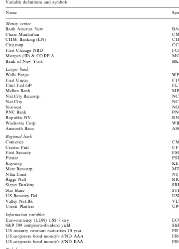
Observations are sampled at weekly intervals. The weekly data ranges from November 6, 1987 to August 28, 1998, which is a 565-data-point series. However, this paper works with rates of return and use the first difference of information variables, and finally all the instruments are used with a one-week lag, relative to the excess return series; that leaves 562 observations expanding from November 27, 1987 to August 28, 1998. Table 1 describes the variables and their symbols used in this paper. All the data are extracted from DATASTREAM.
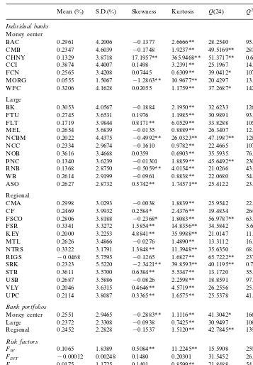
Summary statistics for bank stock returns, risk factors, and instruments used in this paper are presented in Table 2. The mean excess returns for three bank stock portfolios are 0.2551% for Money Center bank, 0.2372% for Large bank, and 0.2452% for Regional bank. These mean excess returns are all greater than 0.1065%, the mean excess return for MSCI world equity index. However, their standard deviations are also greater than that of MSCI world equity index, indicating that investors are compensated for a higher risk premium when holding bank stocks. The positive change in the exchange rate reflects the depreciation of the US dollar against the currencies of ten industrialized countries. The coefficients of skewness and excess kurtosis reveal nonnormality in the data. The last two columns in Table 2 report the Ljung-Box portmanteau test statistics for indepen-dence in the return and squared return series up to 24 lags, denoted by Q(24) and
Q2(24) respectively. The Ljung-Box portmanteau test statistics for independence in
the standardized residuals are calculated using autocorrelations up to 24 lags, and they follow a x2 distribution with 24 degrees of freedom.6The hypothesis of linear
independence is rejected at 5% level for Money Center bank and 1% level for Regional bank. Independence of the squared return series is rejected at 1% level for all three bank portfolio returns, MSCI world equity returns, and the exchange rate changes. Clearly, the nonlinear dependencies are much prevalent than the linear dependencies found in the data and it is consistent with the volatility clustering observed in most financial data: Large (small) changes in prices tend to be followed by large (small) changes of either sign. The GARCH model used in this study is well known to capture this property.
6. Empirical results
6.1. Unconditional test of three-factor model:NLSUR 6ia GMM
Following Ferson and Harvey (1994), this paper first estimates and tests the unconditional three-factor asset pricing model (Eq. (11)) where the expected factor risk premia are assumed to be time-invariant as a restricted nonlinear seemingly unrelated regression model (NLSUR). The NLSUR via Hansen’s (1982) generalized method of moments (GMM), which is valid under weak statistical assumptions, is implemented. To apply the GMM technique, the data used in the estimation must
6The formula for the Ljung-Box statistic isLB(k)=T(T+2) k
j=1rj
2/(T−j), wherer
jis the jth lag
Table 1
Euro-currency (LDN) US$ 7 day ECUSD7D
S&P 500 composite-dividend yield S&PDY
FRTCM10 US treasury constant maturities 10 year
US corporate bond moody’s S’ND AAA FRCBAAA
FRCBBAA US corporate bond moody’s S’ND BAA
Risk factors
MSWRLD MSCI world US$
US treasury constant maturities 10 year FRTCM10
Table 2
Summary statistics of bank stock returns, risk factors and instrumentsa
Mean (%) S.D.(%) Skewness Kurtosis Q(24) Q2(24)
Indi6idual banks
Money center
−0.1377 2.6666**
BAC 0.2961 4.2006 28.2540 95.7098**
CMB 0.2347 4.6039 −0.1748 1.9237** 49.5169** 281.8171** 3.8718
MORG 0.0555 1.5067 −1.2863** 10.9677** 20.4297 13.9133 0.02055 1.1759** 37.2687* 142.5659**
0.2334 −0.1610 0.9782** 22.4665 107.1514** NCC
NOB 0.3616 3.4668 0.0359 0.6903** 35.5935 76.8951**
−0.01301 1.8859** 45.6492**
3.6239 230.4390**
PNC 0.1340
2.8750
0.1368 −0.5059** 4.0154** 21.0266 43.9046** RNB
WB 0.2614 2.9199 −0.0961 0.8838** 22.0680 54.9341** 0.5742** 1.74571** 25.4122 23.6111
0.2806 −0.2368* 1.8083** 56.9787** 63.9084** FSCO
0.2626 −0.0276 1.4890** 13.3112 16.0097 MTL
0.2323 −2.3421** 39.8593** 40.1195** 0.7907 SBK
UPC 0.2114 3.8087 0.3365** 1.6575** 25.5378 41.6411*
Bank portfolios
−0.2883**
Money center 0.2551 2.9465 1.1116** 41.3042* 166.5553** 0.2372 2.3308 −0.0938 0.7425** 30.9497 108.1141** Large
2.2828
0.2452 −0.1537 1.5120** 42.7845** 139.8178** Regional
Risk factors
0.5084**
FW 0.1065 1.8389 11.2245** 15.5908 259.7811**
FINT −0.00012 0.00248 0.1480 0.20301 31.5452 26.6112
Table 2 (Continued)
Q2(24) Skewness Kurtosis Q(24)
Mean (%) S.D.(%)
−0.000018 0.000667 −0.2520** 2.9766** 44.1744* 182.2403** DUSDP
a‘Money Center’ is the equally weighted average of excess returns on 7 individual money center banks. ‘Large’ is the equally weighted average of excess returns on 11 individual large banks. ‘Regional’ is the equally weighted average of excess returns on 13 individual regional banks.FWis the excess return
on the Morgan Stanley world stock total return index in US $. FINT is the log first difference of
FRTCM10. FFX is the log first difference of US$TRDW. SPDIV is the first difference of S&P500
dividend yield in excess of ECUSD7D. DUSTP is the first difference of FRTCM10 in excess of ECUSD7D.DUSDP is the first difference of FRCBBAA in excess of FRCBAAA.Q(24) andQ2(24) are the Ljung-Box test statistics of order 24 for serial correlation in the standardized residuals and standardized residuals squared.
* Denotes statistically significant at the 5% level. ** Denotes statistically significant at the 1% level.
be stationary. As a result, unit root tests are conducted to check if the variables used in the estimation are stationary. The test results not shown here indicate that the null hypothesis of unit root nonstationarity is strongly rejected. The GMM estimator is robust in the sense that one can avoid the usual assumption of homoskedasticity and normality, which are unlikely to hold in these data.7 The
advantage of this approach over the traditional Fama-McBeth approach is that the parameters (l,b) can be estimated jointly and it explicitly allows for contempora-neous correlations across theNassets, and thus is more efficient. A vector of ones and the contemporaneous values of the factor risk s, Fk,t, are used as the
instruments in the GMM. The orthogonality conditions therefore implyE(oitFk,t)=
0 and E(oit)=0, for all i=1, ··· ,Nand k=1, ··· ,K. The estimation results are
presented in Table 3. The unconditional three-factor model is not rejected at 5% level based on the test of overidentifying restrictions (x28
2
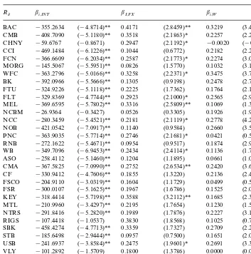
=11.1657 with aP-value of 0.99)8. The estimates of factor loadings (b’s) indicates that almost all banks (27
out of 31) have significant negative factor loadings on interest rate risk at 1% level, 14 banks are sensitive to exchange rate risk, and 20 banks are sensitive to the world market risk. The negative factor loadings on interest rate risk indicate that banks are hurt by unexpected increases in the interest rates. As far as the factor risk premia are concerned, the interest rate risk premium is the only significant factor premium at 5% level with a point estimate of −0.0006%. This negative interest rate risk premium is consistent with previous work of Sweeney and Wagra (1986) and Choi et al. (1992) who use similar approach.
7An alternative approach used by previous researchers (see, e.g., Gibbons, 1982; McElory and Burmeister, 1988; Jorion, 1991; Prasad and Rajan, 1995; Choi and Rajan, 1997; and Choi et al., 1998) is the iterated non-linear seemingly unrelated regression method, which is asymptotically equivalent to maximum-likelihood estimation under the assumption of normality.
Table 3
Unconditional three-factor asset pricing model: NLSUR via GMM estimationa bi,W
bi,INT bI,FX
Rit
−355.2634 (−4.8714)** 0.4171 (2.8459)** 0.3219 (3.4618)** BAC
−366.6609 0.2587 (2.1773)* 0.2274 (3.0163)** FCN
(−5.5951)**
−145.5067 0.0826 (1.5770) 0.1032 (3.1078)**
MORG
0.3258 (2.2371)* 0.3475
(−5.0166)** (3.7614)**
WFC −363.2796
−392.0966 (−5.5666)** 0.1305 (0.9198) 0.2478 (2.7552)** BK
−329.8369 0.2923 (2.1000)* 0.2565 (2.9069)** FLT
(−5.7802)**
−369.6595 0.3316 (2.5809)** 0.1069 (1.3117) MEL
0.0526 (0.3305) 0.1926
(−0.3427) (1.9128)
NCBM −26.9364
(−5.4521)**
−280.3459 0.2181 (2.1119)* 0.2778 (4.2394)** NCC
WB −349.7096 (−6.9453)** 0.2434 (2.4114)* 0.1136 (1.7723) 0.1204 (1.1895) 0.0661
(−5.1460)** (1.0294)
ASO −258.4112
(−7.0990)**
−367.5825 0.2752 (2.6534)** 0.2420 (3.6723)** CMA
(−4.7606)**
−330.9412 0.1855 (1.3220) 0.2136 (2.4033)*
CF
0.1604 (1.1729) 0.0499
(−3.0319)** (0.5763)
FSCO −204.9110
(−5.1625)**
−300.0107 0.1967 (1.6786) 0.1525 (2.0539)*
FSR
−185.6498 0.0957 (0.7500) 0.1651 (2.0438)*
STB
(−3.8584)**
−241.6937 0.2475 (1.9601)* 0.2691 (3.3624)** USB
0.1800 (1.3786) 0.0000
(−1.5709) (0.0004)
VLY −101.2892
UPC −239.7226 (−3.5856)** 0.3995 (2.9676)** 0.1230 (1.4411)
−0.000024 (−0.0107) 0.0024
(−2.1346)* (0.8381)
−0.000006
Test of overidentifying restrictions (J-test):x252 =11.1657 [P-value=0.9980]. ar
it=bi,INT(oINT,t+lINT)+bi,FX(oFX,t+lFX)+bi,W(oW,T+lW)+oit Öi where rit represents the excess
bank stock returns,ok,t’s are the de-meaned values of risk factors,l’s are the risk premia associated with the risk factors, andb’s are the banks’ sensitivities to the risk factors. The instruments in the GMM estimations are a constant and the risk measures. Thex2 test is the minimized values of the GMM criterion function for the system. Robust t-statistics are given in parentheses.
* Indicate statistically significant at the 5% level. ** Indicate statistically significant at the 1% level.
6.2. Conditional tests of three-factor model:pricing kernel approach
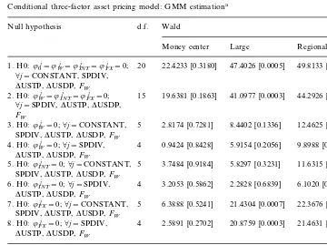
assumed three risk factors can be found, in particular, the world market and exchange rate risks. The conditional three-factor model (Eq. (7)) for each of the three bank types is estimated based on the pricing kernel approach. The empirical results are presented in Table 4.9
As can be seen from the table, the model applied to all three different bank types can not be rejected at any conventional levels based on theJ-test of overidentifying restrictions. Consequently, the hypothesis testing concerning the pricing of risk factors can be conducted. Specifically, a Wald statistic is computed to test the null hypothesis that all8’s coefficients of instrumental variables are zero with respect to a particular risk factor. First, none of the Wald statistics is significant for Money Center bank, indicating that the selected instruments are not useful in predicting risk premia for Money Center bank. However, in contrary to the evidence found
Table 4
Conditional three-factor asset pricing model: GMM estimationa d.f.
4 0.9424 [0.8428] 5.9154 [0.2056] 9.8988 [0.0422] 4. H0:8Wj =0;Öj=SPDIV,
DUSTP,DUSDP,FW
5. H0:8INT
j =0;Öj=CONSTANT, 5 3.7484 [0.9184] 5.8297 [0.3231] 11.6315 [0.0402]
SPDIV,DUSTP,DUSDP,FW
4 2.5891 [0.2702] 20.8759 [0.0003] 21.4631 [0.0003] 8. H0:8FXj =0;Öj=SPDIV,
P-values are in the brackets.
with respect to Money Center bank, significant pricing of time-varying risk factor is detected for Large bank. That is, the joint null hypothesis of constant risk prices is strongly rejected at 1% level based on the Wald test. In particular, the time-vary-ing risk price basically comes from the exchange rate risk because the null hypothesis of constant price of exchange rate risk is rejected at 1% level with a
P-value of 0.0003. Finally, for Regional bank, the joint null hypothesis of constant risk prices is strongly rejected at 1% level with a P-value of 0.0001 based on the Wald test. The time-varying risk prices come from two sources: exchange rate risk and world market risk because the null hypotheses of constant price of exchange rate risk and world market risk is rejected at 1% and 5% level, respectively. In additional, significant price of interest rate risk is detected at 5% level although it is not time varying.
Overall the empirical evidence based on the pricing kernel approach indicates that exchange rate risk is an important risk factor in describing the dynamics of risk premia found in the US bank stock returns, especially for the Large and Regional banks. This evidence of time-varying price of exchange risk is consistent with previous work of Choi et al. (1998) in a domestic context, and of Ferson and Harvey (1993), Dumas and Solnik (1995) and Tai (1999a) in an international context. It may explain why previous researchers are not able to detect significant pricing of exchange rate risk when restricting themselves in an unconditional framework.10
Although the pricing kernel estimation is parsimonious in the sense that re-searchers do not need to specify the dynamics of the conditional second moments, this parsimony also comes with cost. That is its inability to answer questions like ‘‘What does the fitted risk premium look like?’’ and ‘‘What do the fitted conditional covariances look like?’’ To answer these interesting questions, the conditional second moments in the asset pricing models should be explicitly modeled.11
In addition, one would expect the interest rate risk to receive a non-zero price for bank stock returns. Therefore, in the next section a parsimonious parameterization of multivariate GARCH in mean model is employed to explicitly deal with these problems.
6.3. Conditional tests of three-factor model:MGARCH-M
Given the computational complexity of estimating a multivariate system under the GARCH framework, three equally weighted bank stock portfolios are studied, namely those of Money Center bank, Large Bank, and Regional bank. The
10For example, Jorion (1991) tests unconditional multi-factor asset pricing models and fail to find significant evidence of exchange risk pricing in the US stock market. Hamao (1988) also can not find any evidence of exchange risk pricing in the Japanese stock market.
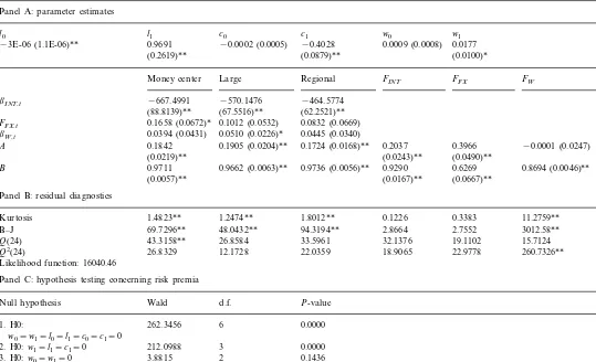
estimation results of conditional three-factor asset pricing model (Eq. (25)) using MGARCH-M approach are presented in Table 5. Panel A reports QML estimates of the parameters for the model. Regarding the factor betas, significant interest rate betas are found for all three bank portfolios at 1% significance level. Consistent with conventional wisdom, bank stock returns are very sensitive to the changes in interest rates, and thus expose to interest rate risk. Exchange rate beta is significant for Money Center bank at 5% level, and for Large bank at 10% level. World market beta is significant for Large bank at 5% level. Finding significant factor betas does not necessarily imply that market participants care about those factor risks because they may be diversifiable, and thus are not priced. To examine whether the chosen three risk factors are priced by the market participants, we test whether the estimated pricing parameters are statistically significant. As can be seen in Panel A, strong evidence of GARCH in mean effects are found for the dynamics of interest rate and exchange rate risk factors since the parameters (l1,c1)are all
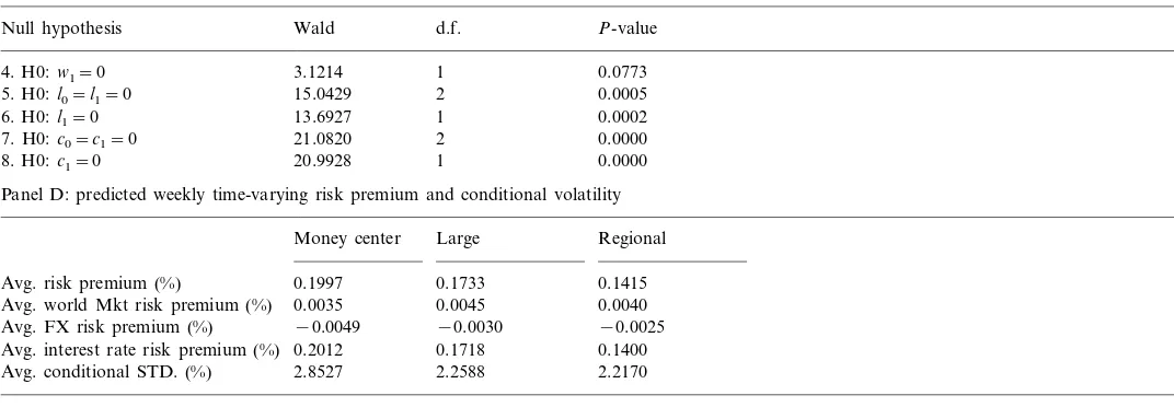
significant at 1% level, and thus it has significant impact on the dynamics of risk premia for the bank portfolio returns. However, the GARCH in mean effect is marginally significant at 10% level for the MSCI world equity index, implying that after accounting for the time-varying interest rate and exchange rate risk premia in asset returns, the world market risk does not play a major role in explaining the dynamics of bank portfolio returns. To further examine the factor risk pricing, we conduct several hypothesis testing in Panel C. For example, the null hypotheses of constant risk premia with respect to interest rate and exchange rate risk factors are strongly rejected at 1% level, and it is rejected at 10% level for the world market risk. The significant evidence of time-varying interest rate, and exchange rate risk premia found in the US bank data points out the advantage of MGARCH-M approach over the previous two approaches. This advantage comes directly from the explicit modeling of conditional volatilities in both asset returns and risk factors, which is ignored in the other two approaches.
Next, consider the estimated parameters for the conditional variance processes. With the exception of parameter a for MSCI world equity index, all the elements in the vectors a andb are statistically significant at 1% level, implying that strong GARCH effect is present for all the return series. In addition, the estimates satisfy the stationarity conditions for all the variance and covariance processes.12
Panel B contains some diagnostic statistics on the standardized residuals (otht
−1/2)
and the standardized residuals squared (ot2h−t 1). With the exception of Money
Center bank, the null hypothesis of linear independency can not be rejected for all the series, as evidenced by the insignificant Ljung Box statistics of order 24 for the standardized residuals (Q(24)). Similarly, the null hypothesis of nonlinear indepen-dency can not be rejected based on the insignificant Ljung Box statistics of order 24 for the standardized residuals squared (Q2
(24)) except for the MSCI world equity index. Overall, the conditional factor asset pricing model with MGARCH-M parameterization effectively eliminates most of the linear and nonlinear
C
Quasi-maximum likelihood estimation of conditional three-factor asset pricing model: multivariate GARCH(1,1)-M Panel A: parameter estimates
−3E-06 (1.1E-06)** 0.9691 −0.4028
(0.0879)**
FFX,t 0.1658 (0.0672)* 0.0832 (0.0669)
0.0510 (0.0226)*
bW,t 0.0394 (0.0431) 0.0445 (0.0340)
0.2037
0.1842 0.1905 (0.0204)** 0.1724 (0.0168)** 0.3966 −0.0001 (0.0247)
A
Q(24) 43.3158** 26.8584 33.5961 32.1376 19.1102 15.7124
260.7326**
26.8329 12.1728 22.0359 18.9065 22.9778
Q2(24)
Likelihood function: 16040.46
C
Panel C: hypothesis testing concerning risk premia
Wald d.f. P-value
Panel D: predicted weekly time-varying risk premium and conditional volatility Money center Large Regional
0.1997 0.1733 0.1415
Avg. risk premium (%)
0.0035 0.0045 0.0040
Avg. world Mkt risk premium (%)
−0.0025 Avg. FX risk premium (%) −0.0049 −0.0030
0.2012 0.1718 0.1400
Avg. interest rate risk premium (%)
Avg. conditional STD. (%) 2.8527 2.2588 2.2170 ar
i,t=(w0+w1hw,t+oW,t)biW+(l0+l1hINT,t+oINT,t)biINT+(c0+c1hFX,t+oFX,t)biFX+oi,t i=Money Center, Large, Regional
FW,t=w0+w1hw,t+ow,t lW,t=E(FW,tVt−1)=w0+w1hw,t FINT,t=l0+l1hINT,t+oINT,t lINT,t=E(FINT,tVt−1)=l0+l1hINT,t FFX,t=c0+c1hFXT,t+oFX,t lFX,t=E(FFX,tVt−1)=c0+c1hFX,t
otVt−1N(0,Ht)
Ht=H0*(ii%−aa%−bb%)+aa%*ot−1o%t−1+bb%*Ht−1
whereHtis a 6×6 conditional covariance matrix of three bank portfolio returns and three risk factors.Q(24) andQ2(24) are the Ljung-Box test statistics
of order 24 for serial correlation in the standardized residuals and standardized residuals squared. B–J is the Bera-Jarque test statistic for normality. Robust standard errors are given in parentheses.
cies found in the raw data. However, the conditional normality assumption is rejected for most cases according to the index of excess Kurtosis and Bera-Jarque test statistics, and that is why QML testing procedures are used.
Because the three-factor asset pricing model with MGARCH-M process is fully parameterized, some interesting statistics can be recovered in this study. Panel D contains those statistics for the estimated time-varying risk premia and conditional volatility. For example, the estimated weekly total time-varying risk premium is 0.1997% for Money Center bank, 0.1733% for Large Bank, and 0.1415% for Regional Bank. We can further decompose the estimated total time-varying risk premium into three components: world market risk premium, foreign exchange risk premium, and interest rate risk premium. For example, the estimated weekly world market risk premium is 0.0035% for Money Center bank, 0.0045% for Large Bank, and 0.004% for Regional Bank. The estimated weekly foreign exchange risk premium is −0.0049% for Money Center Bank, −0.0030% for Large Bank, and
−0.0025% for Regional Bank. Finally, the estimated weekly interest rate risk premium is 0.2012% for Money Center bank, 0.1718% for Large Bank, and 0.14% for Regional Bank. Clearly, the interest rate risk premium is the major component in describing the dynamics of the US bank portfolio returns. Panel D also reports the estimated conditional volatility for each bank portfolio. The estimated weekly conditional volatilities are 2.8527, 2.2587, and 2.2170% for Money Center Bank, Large Bank, and Regional Bank, respectively.
7. Conclusion
returns and bank portfolio returns are considered. The empirical evidence found in this paper can be summarized as follows.
Estimations based on NLSUR via GMM indicate that interest rate risk is the only priced factor in the unconditional three-factor model. However, based on the pricing kernel approach, strong evidence of exchange rate risk is found in both large bank and regional bank stocks, and strong evidence of world market risk is found for the regional bank stocks in the conditional three-factor model with time-varying risk prices. However, no evidence of significant interest rate risk is detected, which is particularly puzzling for the bank stocks. Finally, estimations based on the MGARCH-M approach where both conditional first and second moments of bank portfolio returns and risk factors are estimated simultaneously show strong evidence of time-varying interest rate and exchange rate risk premia and weak evidence of time-varying market risk premium for all three bank portfolios, namely those of Money Center bank, Large bank, and Regional bank. The significant evidence of time-varying interest rate, and exchange rate risk premia found in the US bank data points out the advantage of MGARCH-M approach over the previous two approaches. This advantage comes directly from the explicit modeling of conditional volatilities in both asset returns and risk factors, which is ignored in the other two approaches. Moreover, among the three time-varying risk premia, interest rate risk premium is found to be the major one in describing the dynamics of the US bank portfolio returns.
Acknowledgements
For useful comments and suggestions on earlier drafts, I thank Nelson C. Mark, Paul Evans, G. Andrew Karolyi, Zhiwu Chen, J. Huston McCulloch, Peter Howitt, as well as workshop participants at The Ohio State University and seminar participants at the 1999 FMA Annual Meeting in Orlando, Florida, the 7th Conference on Pacific Basin Finance, Economics and Accounting in Taipei, Tai-wan, ROC, and the 11th Annual PACAP/FMA Finance Conference in Singapore. I also thank the editor, I. Mathur, and an anonymous referee, for their professional critique and suggestions. Any remaining errors are, of course, my responsibility.
References
Bollerslev, T., 1986. Generalized autoregressive conditional heteroskedasticity. J. Econom. 31, 307 – 327. Bollerslev, T., Wooldridge, J.M., 1992. Quasi-maximum likelihood estimation and inference in dynamic
models with time-varying covariances. Econom. Rev. 11, 143 – 172.
Choi, J.J., Elyasiani, E., Kopecky, K.J., 1992. The sensitivity of bank stock returns to market, interest and exchange rate risks. J. Banking Finance 16, 983 – 1004.
Choi, J.J., Hiraki, T., Takezawa, N., 1998. Is foreign exchange risk priced in the Japanese stock market? J. Financial Quant. Anal. 33, 361 – 382.
De Santis, G., Gerard, B., 1997. International asset pricing and portfolio diversification with time-vary-ing risk. J. Finance 52, 1881 – 1912.
De Santis, G., Gerard, B., 1998. How big is the premium for currency risk? J. Financial Econ. 49, 375 – 412.
Ding, Z., Engle, R.F., 1994. Large scale conditional covariance matrix modeling, estimation and testing. UCSD Discussion Paper.
Dumas, B., Solnik, B., 1995. The world price of exchange rate risk. J. Finance 50, 445 – 479. Elyasiani, E., Mansur, I., 1998. Sensitivity of the bank stock returns distribution to changes in the level
and volatility of interest rate: A GARCH-M model. J. Banking Finance 22, 535 – 563.
Engle, R.F., Kroner, K.F., 1995. Multivariate simultaneous generalized ARCH. Econometric Theory 11, 122 – 150.
Engle, R.F., Ng, V.K., Rothschild, M., 1990. Asset pricing with a FACTOR-ARCH covariances structure: Empirical Estimates for Treasury bills. J. Econom. 45, 213 – 237.
Ferson, W.E., 1995. Theory and testing of asset pricing models. In: Jarrow, R.A., Maksimovic, V., Ziemba, W.T. (Eds.), Finance, Handbooks in Operation Research and Management Science, Vol. 9. North Holland, Amsterdam.
Ferson, W.E., Harvey, C.R., 1993. The risk and predictability of international equity returns. Rev. Financial Stud. 6, 527 – 567.
Ferson, W.E., Harvey, C.R., 1994. Sources of risk and expected returns in global equity markets. J. Banking Finance 18, 775 – 803.
Ferson, W.E., Korajczyk, R.A., 1995. Do arbitrage pricing models explain the predictability of stock returns? J. Business 68, 309 – 349.
Flannery, M.J., Hameed, A.S., Harjes, R., 1997. Asset pricing, time-varying risk premia and interest rate risk. J. Banking Finance 21, 315 – 335.
Gibbons, M.R., 1982. Multivariate tests of financial models. J. Financial Econ. 10, 3 – 27.
Hamao, Y., 1988. An empirical examination of the arbitrage pricing theory. Jpn. World Economy 1, 45 – 62.
Hansen, L.P., 1982. Large sample properties of the generalized method of moments estimators. Econometrica 50, 1029 – 1054.
Hansen, L.P., Jagannathan, R., 1991. Implications of security market data for models of dynamic economies. J. Political Economy 99, 225 – 262.
Jorion, P., 1991. The pricing of exchange risk in the stock market. J. Financial Quant. Anal. 26, 362 – 376.
Korajczyk, R.A., Viallet, C.J., 1989. An empirical investigation of international asset pricing. Rev. Financial Stud. 2, 553 – 585.
Korajczyk, R.A., Viallet, C.J., 1993. Equity risk premia and the pricing of foreign exchange risk. J. Int. Econ. 33, 199 – 228.
Koutmos, G., 1997. Is the market portfolio a dynamic factor? Evidence from individual stock returns. Financial Rev. 32, 411 – 430.
Ljung, G.M., Box, G.E.P., 1978. On a measure of lack of fit in time series models. Biometrika 66, 297 – 303.
McElory, M.B., Burmeister, E., 1988. Arbitrage pricing theory as a restricted non-linear multivariate regression model. J. Business Econ. Stat. 6, 29 – 42.
Merton, R.C., 1973. An intertemporal capital asset pricing model. Econometrica 41, 867 – 888. Merton, R.C., 1980. On estimating the expected return on the market: An exploratory investigation. J.
Financial Econ. 20, 323 – 361.
Ng, V.K., Engle, R.F., Rothschild, M., 1992. A multi-dynamic-factor model for stock returns. J. Econom. 52, 245 – 266.
Prasad, A.M., Rajan, M., 1995. The role of exchange and interest risk in equity valuation: A comparative study of international stock markets. J. Econ. Business 47, 457 – 472.
Ross, S.A., 1976. The arbitrage pricing theory of capital asset pricing. J. Econ. Theory 13, 341 – 360. Song, F., 1994. A two-factor ARCH model for deposit-institution stock returns. J. Money Credit
Sweeney, R.J., Wagra, A.D., 1986. The pricing of interest-rate risk: evidence from the stock market. J. Finance 41, 393 – 410.
Tai, C.S., 1998. A multivariate GARCH in mean approach to testing uncovered interest parity: Evidence from Asia-Pacific foreign exchange markets. Unpublished Manuscript, The Ohio State University. Tai, C.S., 1999a. Time-varying risk premia in foreign exchange and equity markets: Evidence from
Asia-Pacific countries. J. Multinational Financial Manage. 9, 291 – 316.
Tai, C.S., 1999b. Market integration, liberalization, and foreign exchange risk in Asia-Pacific emerging markets. Unpublished Manuscript, The Ohio State University.
Tai, C.S., 1999c. Can time-varying price of risk and volatility explain the predictable excess return puzzle in foreign exchange markets. Unpublished Manuscript, The Ohio State University.
Tai, C.S., 2000. On the pricing of foreign exchange risk and risk Exposure in the Japanese stock market. Unpublished Manuscript, The Ohio State University.
Turtle, H., Buse, A., Korkie, B., 1994. Tests of conditional asset pricing with time-varying moments and risk prices. J. Financial Quant. Anal. 29, 15 – 29.
Wetmore, J.L., Brick, J.R., 1994. Commercial bank risk: market, interest rate, and foreign exchange. J. Financial Res. 17, 585 – 596.