Metric Spaces
in Pure and Applied Mathematics
A. Dress, K. T. Huber1, V. Moulton2
Received: September 25, 2001 Revised: November 5, 2001 Communicated by Ulf Rehmann
Abstract. The close relationship between the theory of quadratic forms and distance analysis has been known for centuries, and the the-ory of metric spaces that formalizes distance analysis and was devel-oped over the last century, has obvious strong relations to quadratic-form theory. In contrast, the first paper that studied metric spacesas such– without trying to study their embeddability into any one of the standard metric spaces nor looking at them as mere ‘presentations’ of the underlying topological space – was, to our knowledge, written in the late sixties by John Isbell. In particular, Isbell showed that in the category whose objects are metric spaces and whose morphisms are non-expansivemaps, a uniqueinjective hullexists for every object, he provided an explicit construction of this hull, and he noted that, at least for finite spaces, it comes endowed with an intrinsic polytopal cell structure.
In this paper, we discuss Isbell’s construction, we summarize the his-tory of — and some basic questions studied in —phylogenetic analysis, and we explain why and how these two topics are related to each other. Finally, we just mention in passing some intriguing analogies between, on the one hand, a certain stratification of the cone of all metrics de-fined on a finite setXthat is based on the combinatorial properties of the polytopal cell structure of Isbell’s injective hulls and, on the other, various stratifications of the cone of positive semi-definite quadratic forms defined on Rn that were introduced by the Russian school in
the context of reduction theory.
2000 Mathematics Subject Classification: 15A63, 05C05, 92-02, 92B99
1
The author thanks the Swedish National Research Council (VR) for its support (grant# B 5107-20005097/2000).
2
Keywords and Phrases: injective hull, tight span, phylogenetic tree, quadratic form
1 Introduction
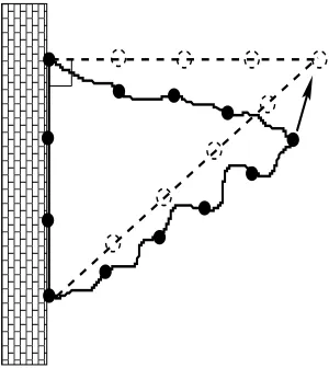
The close relationship between distance analysis and quadratic-form theory was known already in pre-Pythagorean times: A ceramic slab found in the near east, for instance, presents the triples of integers 3,4,5; 5,12,13; 7,24,25; ... and it is very likely that these integers were of interest to Babylonean builders as they allowed to build walls at right angles without any particular tool except a long string with 12 = 3+4+5 or 30 = 5+12+13 or ... equidistant nodes (see Figure 1).
Figure 1: The figure shows how a wall can be built at a right angle with a string of length 12.
The Pythagorean Theorem puts this knowledge into more formal terms. And since then, the analysis of distance relationships has always been closely intertwined with that of quadratic forms. The development of differential geometry since Gauss as well as the development of geometric algebra in the 19th century — culminating in the definition of Clifford and Cayley algebras and Hamilton’s definition of quarternian fields — clearly testifies to this fact.
spaces as just a rather convenient tool to define and to deal with topological spaces, a few began to study metric spaces for their own sake. Menger and Blumenthal in particular began developing distance geometry providing and investigating necessary and sufficient conditions for a given metric space to be isometrically embeddable into standard metric spaces, e.g. the n-dimensional Euclidean or some hyperbolic, elliptic, orLpspace — rediscovering, by the way,
an important result of Cayley’s regarding the significance of the now famous Cayley-Menger determinantsin this context3. While, at their time, this effort did not stimulate much of a response among their fellow mathematicians, it turned out to be crucial later on for developing algorithms that would identify the spatial structure of proteins fromtwo-dimensionalNMR data (cf. [7]).
2 John Isbell’s Contribution
Perhaps the first paper that studied metric spacesas such– without trying to study their embeddability into standard metric spaces nor looking at them as mere ‘presentations’ of the underlying topological space – was, to our knowl-edge, written in the late sixties by John Isbell (cf. [23]). Trying to capture the decisive aspects of distance relationships, he proposed to define thecategory of metric spacesas follows: Its objects — for sure — are the metric spaces. But, noting that
• using continuous maps as morphisms would create too flexible a category, overemphasizing the topological aspects and neglecting the true metric structure (e.g. any bijection between two finite metric spaces would then be an isomorphism)
while
• using isometries only would result in too rigid a category without enough morphisms,
he proposed to use thenon-expansivemaps from a metric spaceAinto a metric spaceB as the set of morphisms fromAto B, that is, those mapsf :A→B
for which the distance in B between the image f(a) and f(a′
) of two points
a and a′
from A never exceeds their distance in A (or, in other words, the continuous maps fromAtoBfor which the Weierstrassδcan always be chosen to be equal to the Weierstrassε).
Isbell then went on to show that a uniqueinjective hullexists in this category for every one of its objects, providing an explicit construction of this hull for all spaces and noting that it comes endowed, at least for finite spaces, with an
3
intrinsic polytopal structure.
More precisely, Isbell presented the following intriguing observations:
(i) There exist injectivemetric spaces, that is, metric spaces X = (X, d) = (X, d:X×X →R) such that, for every isometric embeddingα:X ֒→X′
of (X, d) into another metric space (X′, d′), there exists a non-expansive
retract α′ : X′ → X, that is, a non-expansive map α′ from X′ into X
withα′
◦α=IdX.
(ii) Every metric space (X, d) can be embedded isometrically into an injective metric space ( ˆX,dˆ).
(iii) Given any such isometric embeddingα:X ֒→Xˆ of a metric space (X, d) into an injective metric space ( ˆX,dˆ), there exists a unique smallest injec-tive subspace ( ¯X,d¯) of ( ˆX,dˆ) containing α(X). This subspace depends – up to isometry – only on (X, d):
• The map
¯
X→RX : ¯x7→(hx¯:X →R:x7→d¯(α(x),x¯))
is easily seen to define an isometric embedding of ¯X into the setRX
of all maps from X into R endowed with the supremum norm (or
l∞metric)
||f, g||∞:= sup(|f(x)−g(x)|:x∈X) (f, g∈R
X).
• And its image consists exactly of all those mapsf ∈RX that satisfy the condition
f(x) = sup(d(x, y)−f(y) :y∈X)
for allx∈X}.
In [9], this subset of RX has also been called the tight span T(X, d) of (X, d) — a tradition that we will follow is in this paper, too.
(iv) In addition, the above embedding identifiesX with the set
{hx:X →R:y7→d(y, x) :x∈X}
and, hence, with the subset
T0(X, d) :={f ∈T(X, d) : 0∈f(X)}
(v) The above definition/construction of T(X, d) identifies it with a subset of the convex set
P(X, d) :={f ∈RX :f(x) +f(y)≥d(x, y) for all x, y∈X},
more precisely, it identifies it with the set of allminimalmaps inP(X, d) (relative to the partial orderP(X, d) inherits from the partial order of
RX defined, as usual, byf ≤g ⇐⇒ f(x)≤g(x) for allx∈X). Thus, it
consists of a locally finite collection of (low-dimensional) faces ofP(X, d) whenever this convex set is actually a convex polytope (i.e. determined by a ‘locally finite’ collection of half spaces) which is surely the case ifX
itself is finite.
(v) T(X, d) is always contractible. More precisely, there exists always a con-tinuous familyft (t∈[0,1]) of non-expansive maps
ft:T(X, d)→T(X, d)
withf0=IdT(X,d) and #f1(T(X, d)) = 1.
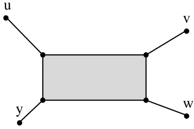
Although these notions may appear to be somewhat strange at first, the tight span of small metric spaces (X, d) can be described in simple geometric terms as follows: In case X consists of just two points of distancec, its tight span is exactly the interval of length c, its end points being just the two points from X (thus the name “tight span”). In caseX consists of just three points of distance c1, c2, c3, its tight span is the union of three intervals of length (c1+c2−c3)/2, (c1+c3−c2)/2,and (c2+c3−c1)/2, respectively, all identified at one end point while the other three end points are the three points fromX. In Figure 2, we picture the tight span of a generic 4-point metric space: In general, the tight span of afinitemetric space (X, d) coincides exactly with the union of all compact faces of the polytope P(X, d). Using this fact, it is possible to determine the polytopal structure of the tight span for a generic metric space of cardinality up to 5, cf. [9]. For finite metric spaces of larger cardinality, it is also possible in principle to determine their tight span, though it can be a tricky combinatorial problem to do this explicitly for any particular given metric space (see e.g.[11, 20]).
It is worthwhile to note that Isbell’s construction does not really need ametric
dto perform its task. It also works just as well forevery mapD from the set
Pfin(X) of all finite subsets of a setX intoR:=R∪ {−∞}(rather than only the mapD=Dd:Pfin(X)→Rdefined byD(Y) :=d(x, y) in caseY ={x, y}
for some x, y in X, and D(Y) :=−∞else): Indeed, if such a mapD is given, we may define
P(X, D) :={f ∈RX: X
x∈Y
f(x)≥D(Y) for allY ∈ Pfin(X)}
and
y
u
w
v
Figure 2: The tight span of a generic metricdon the set{u, v, w, y}for which
d(u, w) +d(v, y) is the largest of the three sums d(u, w) +d(v, y), d(u, v) +
d(w, y), and d(u, y) +d(v, w); it consists of eight 0-cells, eight 1-cells, and one 2-cell.
{f ∈RX:f(x) = sup(D(Y ∪ {x})−X
y∈Y
f(y)) for allY ∈ Pfin(X− {x})}
just as before (so thatP(X, Dd) =P(X, d) andT(X, Dd) =T(X, d) holds for
every metric dand the map Dd associated with it according to the definition
above). It is then not too difficult to establish, in this much more general setting, most of the results collected above in the special case considered originally by John Isbell.
Perhaps a bit surprisingly, this generalization can be used to construct affine buildings ofGL-type. Assume thatK is field with a valuation
val :K→R
that satisfies the usual conditions
(i) val(x) =−∞ ⇐⇒ x= 0,
(ii) val(xy) = val(x) + val(y),
(iii) val(x+y)≤max(val(x),val(y))
for allx, y∈Kand consider, for some natural numbern, the setX :=Knand
the mapD:Pf in(X)→Rdefined by
D(Y) := val(det(x1, ..., xn))
ifY ={x1, ..., xn}andn= #Y, and
else (Y ∈ Pfin(X)). Then, it is easily seen that T(X, D) coincides — together with its induced polytopal structure – with the affine building associated with
GL(n, K) provided the valuation in question is discrete while, in general, it provides at least a useful generalization that should also coincide with generalizations proposed so far for non-discrete valuations [15].
We expect that, in addition, the following example is of relevance in the context of symplectic and orthogonal groups: Let X be any vector space over K on which a sesqui-linear formh · | · ifromX×XintoKis defined and assume that
h · | · iis also “almost symmetric” (i.e. thathx|yi= 0 ⇐⇒ hy|xi= 0 holds for allx, y inX). It is then easy to see that the mapD defined by
D(Y) := val(det(hxi|xji)i,j=1,... ,n)
ifY ={x1, . . . , xn}andn= #Y holds, defines indeed a well-defined map from
Pfin(X) intoRto which Isbell’s construction can be applied. We have not yet checked, but expectT(X, D) to coincide with the corresponding affine building of the symplectic groupSp(2n, K) ifX is of dimension 2nand the formh · | · iis non degenerate and skew-symmetric. We are not so sure about what happens in case h · | · iis non degenerate and symmetric. But we know, of course, that Isbell’s construction at least provides in any case a nice contractible space on which the symmetry group of (X,h · | · i) acts in a canonical fashion (cf. [9]).
3 Phylogenetic Analysis
Isbell’s construction was rediscovered in 1982 (see [9]) when the process of (re)constructing phylogenetic trees from distance data was scrutinized to develop methods for checking the suitability of data for and to improve the reliability of phylogenetic analysis (and, curiously enough, it was rediscovered again in 1994 in a completely different context, cf. [6]).
The goal of phylogenetic analysis is to derive a complete, consistent and, hopefully, true picture of the evolutionary branching process that produced a class of present — and, sometimes also some extinct — species from their last common ancestor, e.g. the evolution of all the various forms of tetrapodes from the firstamphibia-like beings crawling out of the sea around 400 million years ago.
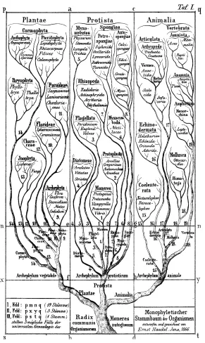
The first such phylogenetic tree encompassing all plant and animal kingdoms then known was constructed in 1866 (see Figure 3) just seven years after the publication, in 1859, of Charles Darwin’s (1809-1882) The Origin of Species4 by the German biologist Ernst Haeckel (1834-1919), the most ardent supporter of Darwin in that time in Germany. While Darwin never made much effort
4
to construct phylogenetic trees explicitly (even though he was, of course, fully aware that his theory implies the existence of such a tree and remarked “As we have no record of the lines of descent, the pedigree can be discovered only by observing the degrees of resemblance between the beings which are to be classed”), it was not too difficult for Ernst Haeckel to design his tree. All he had to do was to give aDarwiniandynamic interpretation of the static systems previously put forward (in form of tableaux) by Carolus Linnaeus (1707-1778), Georges Cuvier (1769-1832) and others.
Linnaeus had become famous very early in his life for his analysis of gender in plants, thus recognizing an amazing universality of certain basic laws of life in the then known living world. In hisSystema Naturae, Sive Regna Tria Naturae Systematice Proposita5, published in 1735 in Leiden, Linnaeus followed the most rigorous scientific traditions of his time. These had been established by John Ray (1628-1705) in his writings since 1660, culminating in hisMethodus Plantorum Nova from 1682 and his posthumously publishedSynopsis Avium et Pisciumfrom 1713. Ray was probably the first scientist to recognize and to conceptualize theinvarianceof species as the fundamental basis of life science. Linnaeus followed Ray’s insights and constructed a whole binary hierarchyof phyla, kingdoms, genera, families, subfamiliesetc. to classify biological species according to their intrinsic similarities.
These ideas were then taken up by scientists like August Quirinus Rivinus (1652-1723) in Germany and Joseph Pitton de Tournefort (1656-1708) in France as well as, a little later, by Linnaeus in Sweden. Like Ray, Linnaeus insisted that the living world (except for a few species doomed by the great deluge and documented in the fossil record) had been created in that very order in which it presents itself to us today and that the task of taxonomy was to search for a “natural system” that would reflect the Divine Order of creation. Darwin’s ideas allowed to reinterpret Linnaeus’ classes as clades, i.e. as collections ofallthose species derived fromonecommon ancestor. Thus, the static Linnaean system could immediately be transformed into Haeckel’s dynamic tree.
However, there are always many details in such trees that are hotly debated, and the evidence that can be used for tree (re)construction is often scarce, inconsistent and contradictory. For instance, it is not yet fully known whether themonotremata— the Australianduck-billed platypusand thespiny anteaters (echidna aculeataandechidna Bruynii) — are more closely related to the mar-supalia (opossums, kangaroos, etc.) than to us (the placental mammals or eutheria) or whether, the third alternative, the placental mammals and the marsupalia are more closely related to each other than both are to the platypus and the echidnas (even though the most recent molecular data appears to
sup-5
port the first alternative). And even less clear are at present the phylogenetic relationships among the various groups of placental mammals (cf. [28] and also http://phylogeny.arizona.edu/tree for fascinating up to date information regarding the present view of Haeckel’s Tree of Life6).
Consequently, biologists have always been looking for further evidence – in addition to morphological evidence, from all parts of the organism in all stages of its development, and metabolic peculiarities – on which phylogenetic con-clusions could be based. So, when the amino acid sequence of closely related proteins from distinct species (and encoded by related though not identical genes all supposedly derived fromonecommon ancestral gene by accumulating successive mutations) became known in sufficient abundance in the late 1960’s, some biologists realized quickly that such documents of molecular evolution might provide the most convincing evidence on which to build phylogenetic trees.
The first paper exploiting this idea that appeared in Science was written by Walter Fitch and Emanuel Margoliash almost thirty five years ago. It was entitled simply Construction of Phylogenetic Trees (cf. [19]) and it caused a revolution in taxonomy. It used the amino acid sequences of cytochrom C, a protein of decisive importance in oxygen metabolism in all eucariots, derived from more than 20 species from all eucariot kingdoms. Fitch and Margoliash estimated the genetic distance d(S1, S2) between any two of these sequences
S1 andS2in terms of the easily computed number of mismatches betweenS1 andS2 relative to amultiple alignmentof all of the sequences in question that had been constructed simply by hand — in this specific case a comparatively simple task in view of the large overall similarity of the sequences.
They then constructed their tree automatically by employing the following very simple standard algorithm from cluster-analysis textbooks:
Given a finite set X together with a symmetric map d from X ×X into R, one defines the setV(X, d) of nodes of the treeTF&M(X, d) to be constructed
to consist of those subsets Y of X that constitute, for some real number c, a connected component of the graph Γc := (X, Ec) whose vertex set is the
given setX and whose edges consist of all pairs of elementsx, y fromX with
d(x, y)≤c. And two such nodesY1, Y2 are connected by an edge if and only if Y1 ⊂ Y2 holds and there is no Y in V(X, d) with Y1 ⊂ Y ⊂ Y2 — or, equivalently, if #{Y ∈V(X, d) :Y1⊆Y ⊆Y2}= 2 holds.
At that time, most taxonomists were appalled by this approach. The definitive result of a scholar’s whole life of research could apparently now be produced in less than a minute by an insightless machine. Others, impressed by the obvious potential of this new approach (which had almost simultaneously also been conceived independently by at least one further research group) took
6
immediately to the road to visit the authors of that paper.
Today, essentially every paper dealing with phylogenetics offers trees produced automatically from sequence data by appropriate computer programs. It also became obvious in the mean time that such trees are not the end of scientific investigation in taxonomy. Rather to the contrary, it needs the full knowledge and expertise of experienced scientists to discuss the computer-generated trees and to point out their weak as well as their strong points.
Clearly, the obvious idea any tree-reconstruction algorithm must use is that, given any three sequences that have been derived by the process of replication, mutation, and selection from one common ancestral sequence, the last com-mon ancestral sequence of the two more similar acom-mong those three sequences should have existed later than the last common ancestral sequence of all three sequences. This suggests the following tree-construction algorithm: First, identify each sequence S from the set X of sequences in question with the corresponding one-element clade {S} consisting of S, only. Then, using any appropriately defined dissimilarity measured:X×X→R(e.g. the mismatch orHammingdistance employed by Fitch and Margoliash), search for those two sequencesS1, S2that have minimal dissimilarity and, supposing that no other sequence in X can be an offspring of the last common ancestral sequence of
S1 andS2, fuse S1 and S2 into one larger d-clade {S1} ∪ {S2}. Then replace the set X by a smaller set X′ representing all maximal, presently identified
(d-)clades (that is, the oned-clade of cardinality 2 and the additional, not yet processed single-element clades at that stage) and define a new dissimilarity measure on those clades by defining the distance d(Y1, Y2) of any two such clades Y1, Y2 to be some function of the dissimilarities d(y1, y2) withy1 ∈Y1 and y2 ∈ Y2. And then, repeat the above process to identify the next two clades that are to be fused into one new, largerd-clade, and so on. Obviously, if d(Y1, Y2) is defined byd(Y1, Y2) := min{d(y1, y2)|y1 ∈Y1, y2 ∈ Y2} for any two d-clades Y1, Y2, this will lead exactly to the tree TF&M(X, d) described
above.
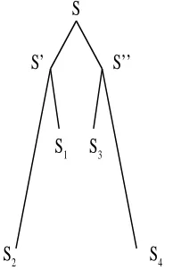
However, this procedure is obviously bound to make mistakes: Assume, we have four sequencesS1, S2, S3, S4 and that, during the evolution of those four sequences from their common ancestor sequenceS, there were first two distinct offsprings sequences S′, S′′ of S so that S
1 and S2 were later derived fromS′ and S3 and S4 from S′′. Assume furthermore that S1 remained very similar to S′ and S
3 remained very similar toS′′ andS2 as well as S4 diverged very far from their respective ancestor sequences. Then, the above algorithm will inevitably form a wrong clade {S1, S3}(see Figure 4).
S
S
2S
4S’
S’’
1
S
S
3Figure 4: As explained in the text, the incorrect clade {S1, S3} is formed by the agglomeration algorithm and the ’true topology’ of the tree is not found.
whose leaves are labeled by the elements from X, and to whose branches appropriate edge lengths are attached so that the resulting inducedtree metric (that associates to any pair of elements x, y from X the total length of the unique path from the two leaves labeled with x and y) matches the given dissimilaritiesin toto as closely as possible.
To imagine the task one has to perform using the approach it is worthwhile to observe that thespaceof all possible dissimilarities that can be defined on an
n-set X has dimension ¡n
2
¢
while the subspace oftree-like dissimilarities that can be defined on X has dimension 2n−3 (the maximal number of branches in a tree with n leaves) and forms a rather complex low-dimensional network of large codimension¡n
2
¢
4 Tree Reconstruction and the Tight Span
Nevertheless, this approach suggests a number of interesting, purely mathe-matical questions which to pursue might still be helpful in this context: E.g., it leads to the question which dissimilarities aretree likedissimilarities, i.e. which dissimilarities would fit exactly into a tree, and whether that tree would be completely determined by those dissimilarities. Fortunately, these two ques-tions have simple answers that have been discovered in the sixties and seventies of the last century independently by various mathematicians (cf. [5, 29, 30]):
(i) A dissimilarity dis tree like if and only if
d(x, y) +d(u, v)≤max{d(x, u) +d(y, v), d(x, v) +d(y, u)}
holds for allx, y, u, v fromX.
(ii) If this condition is fulfilled, there is only one tree that fits the given dissimilarity (up to isomorphism, and except for additional branches not involved with the given data).
Remarkably, once we define a metric on all points of that tree (whether a branching point, an end point, or just a point somewhere on some branch) by associating again to any two such points x, y the total length of the unique path from x to y, the resulting metric space, necessarily an R−tree (by the very definition of R−trees) actually coincides with the injective hull of the metric defined on its leaves. This establishes not only the uniqueness of the tree in question; it can also be used to study the structure of that tree in terms of the metric defined on its leaves. More importantly, it suggests to use the injective hull in any case, whether or not the input dissimilarities satisfy the above four-point condition, as a good substitute for the tree in question — at least, it is always simply connected (though not always of dimension one).
In particular, if there exists some subset K of small diameter within this injective hull T not containing any leaf, yet such that its complementT −K
has several connected components, the (labels of the) leaves in at least all but one of these components have a good chance to form one of those clades within
X that phylogenetic analysis is designed to find.
It was exactly this observation which lead to the rediscovery of Isbell’s construction in 1982 mentioned above. And it also motivated and initi-ated many further investigations regarding the structure of injective metric spaces and their relevance in phylogenetic analysis (cf. [10, 11, 13, 14]). In particular, the analysis of injective hulls of finite metric spaces made it obvious that the injective hull of a sum d = d1+d2+. . .+dk of k metrics
d1, d2, . . . , dk defined on a finite set X is closely related to that of the
sum-mands d1, d2, . . . , dk provided these metrics form a coherent decomposition
f(x) +f(y)≥d1(x, y) +d2(x, y) +. . .+dk(x, y) for all x, y ∈X, some maps
f1, f2, . . . , fk :X →Rsuch that fi(x) +fi(y)≥di(x, y) holds for allx, y∈X
and for alli= 1,2, . . . , k (cf. [2, 24, 25, 26]).
Moreover, defining a metricdto be
- asplit — or acut— metric if there are exactly two subsets ofX in the setX/dof equivalence classes of elements ofX relative to the equivalence relation≃defined onX byx≃y⇔d(x, y) = 0, and
- asplit-primemetric if it cannot be decomposed into a coherent sum of a split metric and another metric,
it could be shown that
- every metricddefined on a finite setX has a unique coherent decompo-sition — also called thecanonical split decompositionof d— into a sum
d=d1+d2+. . .+dk+d0 of pairwise linearly independent split metrics
d1, d2, . . . , dk and a split-prime metricd0 (possibly the 0-metric),
- the metricsd1, d2, . . . , dk occurring in this decomposition are always
lin-early independent (as elements in the vector space of all maps fromX×X
intoR) — and so ared1, d2, . . . , dk, d0 ifd06= 0 holds,
- the metrics d1, d2, . . . , dk occurring in this decomposition are – up to
scaling – exactly those split metricsd′ defined onX for which d−d′ is
also a metric and the two metricsd′, d−d′form a coherent decomposition
ofd,
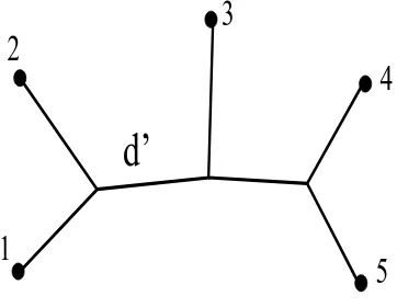
- ifdis a tree-like metric, then the split-prime metricd0in the correspond-ing canonical coherent decomposition d = d1+d2+. . .+dk+d0 of d into a sum of pairwise linearly independent split metrics d1, d2, . . . , dk
and a split-prime metricd0vanishes while the split metricsd1, d2, . . . , dk
correspond in a one-to-one fashion to the branches of the associated tree (cf. Figure 5).
This was of considerable interest within the context of phylogenetic analysis: If a split metricd′ occurs as a summand in a coherent component of a metric dderived from a family of phylogenetically related sequences, there is a good chance that at least one of the two equivalence classes in X/d′ is one of those
clades within X that we want to find.
In particular, given any metricddefined on a setX of cardinalityn, the linear independence of the split metrics occurring in the canonical decomposition of
dimplies that there exist, up to scaling, at most¡n
2
¢
split metricsd′
such that (i) d−d′
is also a metric and (ii) the two metrics d′
, d−d′
1
2
3
4
5
d’
Figure 5: A tree with leaves labeled by the finite set {1,2,3,4,5}. The branch separating the vertices1,2from the vertices3,4,5corresponds to a split metric
d′
withX/d′
={{1,2},{3,4,5}}.
metrics that, up to scaling, can be defined on ann-set.
In addition, it might even be helpful when analyzing a given data set to realize that several competing evolutionary interpretations of the data are possible (as indicated by the existence of two split metrics d′
, d′′
in the canonical decomposition ofdfor which #(X/(d′
+d′′
)) = 4 holds) or that, at least, some additional feature (e.g. some sort ofconvergence) might be present in the data.
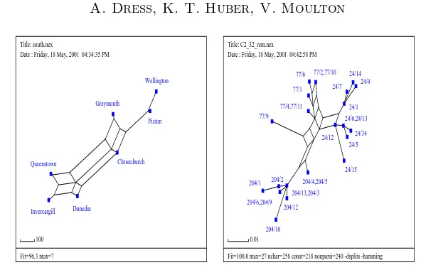
Consequently, algorithms were developed to compute, given any metric D, all split metrics d for which the above conditions are fulfilled as well as to visualize the resulting split network (cf. [3, 12, 22]). The resulting SplitsTree program has proven useful in diverse phylogenetic applications. Moreover, as Figure 6 shows, it can as well be applied to all sorts of distance data: The split networks in Figure 6(left) was computed for the distances between the towns of Wellington on the North Island, and Christchurch, Greymouth etc. on the South Island of New Zealand that were taken from a mileage chart. If one compares this graph with a map of New Zealand a good correlation between the distribution of vertices and the geographical locations of the towns is observed. It has also been applied to analyze the perceived similarity of colors and — instemmatology — the “kinship” relations between the various hand-written versions of Chaucer’s Canterbury tales written by Geoffrey Chaucer about 100 years before book printing was invented (in central Europe) (cf. [4]).
Title: south.nex
Date : Friday, 18 May, 2001 04:34:35 PM
Fit=96.3 ntax=7 Date : Friday, 18 May, 2001 04:42:58 PM
Fit=100.0 ntax=27 nchar=258 const=218 nonparsi=240 -dsplits -hamming
204/1
Figure 6: Split networks for a mileage chart of New Zealand (left) and a hepatitis C virus data set (right).
biology, non tree-like distances often arise when analyzing viral data sets, a phenomenon that is probably caused by more complex evolutionary processes such as recombination. In Figure 6 (right), we present a split network that was computed for a hepatitis C data set which was presented in [1]. In this graph, a complex relationship between various viral sequences (represented by the labeled vertices) is observed. However, there is a clear separation between the three sets of vertices labeled with prefixes 204, 77, and 24, and indeed this reflects the fact that the viruses corresponding to vertices prefixed by 204 and 77 were taken from recipients of blood transfusions from a donor who was infected with the viruses corresponding to the vertices prefixed by 24.
For more applications of the SplitsTree program to biological data see e.g. [8, 12, 16, 21, 27]. The latest version of SplitsTree, written by Daniel Huson, can be obtained from:
http://www.mathematik.uni-bielefeld.de/∼huson
There is also a www version of the program running at:
http://bibiserv.techfak.uni-bielefeld.de/splits
Some further references and discussions of related topics can be found on the following www pages:
and further phylogenies by Haeckel can be found on the following web pages:
http://www.boga.ruhr-uni-bochum.de/spezbot/Folien/ Abb1 Stammbaum Haeckel.html
http://genome.imb-jena.de/stammbaum.html
5 Back to Mathematics and Quadratic forms
In addition to these applications, there are also striking analogies between split-decomposition theory and the theory of positive semi-definite quadratic forms as developed by the Russian school: In both fields, one considers a large convex cone (either consisting of all metrics defined on a finite set or consisting of all positive semi-definite quadratic forms defined on some finite-dimensional vector space), one has good reasons to decompose this cone — in one way or the other — into a family of finitely generated convex subcones, and one wants to understand the combinatorics of the resulting stratification of the large cone. In split-decomposition theory, it is the concept of coherence that gives rise to the stratification in question: given any two metrics d and d′,
defined on a fixed finite setX, one may define the metricd′ to be acoherent
specialization of the metric d if there exists some positive real number ρ
such that d′′ := ρd−d′ is also a metric and the two metrics d′, d′′ form a
coherent decomposition of d. One can show that, given any metricd defined onX, the collection of metricsd′ that are coherent specializations ofdforms
a finitely generated convex subcone C(d) of the cone of all metrics defined on X. Moreover, some (not at all obvious) conditions on d are known from split-decomposition theory which imply that C(d) is a simplicial cone while this does not seem to hold in general for every metricd.
Very similar problems have been (and still are being) studied in the theory of positive semi-definite quadratic forms while trying to understand the process of reduction of quadratic forms (cf. [17, 18]). And in both areas, the extremals of the convex cones in question — the positive semi-definite quadratic forms of rank one on the one hand and the split metrics as well as some further, not yet well understood metrics on the other — appear to be of special significance.
Thus, it might prove rather useful trying not only to develop both theories in parallel, but also to understand the deeper reason for the striking analogy between them.
References
[1] J. -P. Allain, Y. Dong, A. -M. Vandamme, V. Moulton, M. Salmei, Evolu-tionary rate and genetic drift of hepatitis C virus are not correlated with the host immune response: studies of infected donor-recipient clusters, Journal of Virology74(2000) 2541–2549.
[2] H. -J. Bandelt, A. Dress, A canonical decomposition theory for metrics on a finite set, Adv. in Math. 92(1992) 47–105.
[3] H .-J. Bandelt, A. Dress, Split decomposition: a new and useful approach to phylogenetic analysis of distance data, Molecular Phylogenetics and Evolution1(3) (1992) 242–252.
[4] A. C. Barbrook, C. J. Howe, N. Blake, P. Robinson, The phylogeny of The Canterbury Tales, Nature394(1998) 839.
[5] P. Buneman, The recovery of trees from measures of dissimilarity. In F. Hodson et al., Mathematics in the Archaeological and Historical Sci-ences, (pp.387–395), Edinburgh University Press, 1971.
[6] M. Chrobak, L. Lamore, Generosity helps or an 11-competitive algorithm for three servers, Journal of Algorithms16(1994) 234–263.
[7] G. M. Crippen, T. F. Havel, Distance Geometry and Molecular Confirma-tion, Wiley, Chinchester, 1981.
[8] J. Dopazo, A. Dress, A. von Haeseler, Split decomposition: A technique to analyze viral evolution, PNAS90(1993) 10320–10324.
[9] A. Dress, Trees, tight extensions of metric spaces, and the cohomological dimension of certain groups: A note on combinatorial properties of metric spaces, Adv. in Math. 53(1984) 321–402.
[10] A. Dress, K. T. Huber, V. Moulton, A comparison between the median and the tight-span completion of finite split systems, Annals of Combinatorics, 2, 1998, 299–311.
[11] A. Dress, K. T. Huber, V. Moulton, An explicit computation of the injec-tive hull of certain finite metric spaces in terms of their associated Bune-man complex, Advances in Mathematics, to appear.
[12] A. Dress, D. Huson, V. Moulton, Analyzing and visualizing distance data using SplitsTree, Discrete Applied Mathematics71(1996) 95–110. [13] A. Dress, V. Moulton, M. Steel, Trees, taxonomy and strongly compatible
multi-state characters, Advances in Applied Mathematics19(1997) 1–30. [14] A. Dress, V. Moulton, W. Terhalle, T-theory: An overview, European
Journal of Combinatorics17(1996) 161–175.
[15] A. Dress, W. Terhalle, The tree of life and other affine buildings. Proceed-ings of the International Congress of Mathematicians, Vol. III (Berlin, 1998). Doc. Math. 1998, Extra Vol. III, 565–574.
[16] A. Dress, R. Wetzel, The human organism - A place to thrive for the immuno-deficiency virus, in Proceedings of IFCS, Paris.
[18] R. M. Erdahl, Zonotopes, dicings, and Voronoi’s conjecture on parallelohe-dra, European J. Combin.20(1999) 527–549.
[19] W. M. Fitch, E. Margoliash, Construction of phylogenetic trees, Science
155(1967) 279–284.
[20] O. Goodmann, V. Moulton, On the tight span of an antipodal graph, Dis-crete Mathematics218(2000) 73–96.
[21] E. Holmes, M. Worobey, A. Rambaut, Phylogenetic evidence for recombi-nation in dengue virus, Mol. Biol. Evol.16(3) (1999) 405–409.
[22] D. Huson, SplitsTree: a program for analyzing and visualizing evolutionary data, Bioinformatics14(1) (1998) 68–73.
[23] J. Isbell, Six theorems about metric spaces, Comment. Math. Helv. 39
(1964) 65–74.
[24] J. Koolen, V. Moulton, A note on the uniqueness of coherent decomposi-tions, Advances in Applied Mathematics19(1997) 444–449.
[25] J. Koolen, V. Moulton, U. Toenges, The coherency index, Discrete Mathe-matics192(1998) 205–222.
[26] J. Koolen, V. Moulton, U. Toenges, A classification of the six-point prime metrics, European Journal of Combinatorics21(2000) 815–829.
[27] P. Plikat, K. Nieselt-Struwe, A. Meyerhans, Genetic drift can dominate short-term HIV-1 nef quasispecies evolution in vitro, Journal of Virology
71(1997) 4233–4240.
[28] D. Penny, M. Hasegawa, The platypus put in its place, Nature387(1997) 549–550.
[29] J.M.S. Sim˜oes-Pereira, A note on tree realizability of a distance matrix, J. Comb. Theory (B)6 (1969) 303–310.
[30] K.A.Zaretsky, Reconstruction of a tree from the distances between its pendent vertices, Uspekhi Math. Nauk, Russian Mathematical Surveys20
(1965) 90–92 (In Russian).
A. Dress
FSPM-Strukturbildungsprozesse University of Bielefeld
D-33501 Bielefeld, Germany [email protected]
K. T. Huber
FMI, Mid Sweden University S 851-70 Sundsvall
Sweden
V. Moulton
FMI, Mid Sweden University S 851-70 Sundsvall
Sweden