HOW MANY HIPPOS (HOMHIP): ALGORITHM FOR AUTOMATIC COUNTS OF
ANIMALS WITH INFRA-RED THERMAL IMAGERY FROM UAV
S. Lhoest *, J. Linchant **, S. Quevauvillers, C. Vermeulen, P. Lejeune
Forest Resources Management Axis, Biosystems engineering (BIOSE),
University of Liège – Gembloux Agro-Bio Tech, Passage des Déportés, 2 – 4350 Gembloux, Belgium *[email protected], **[email protected], co-first authors
KEY WORDS: Hippos, UAV, Infra-red, Thermal-imagery, Automatic count, Algorithm, QGIS
ABSTRACT:
The common hippopotamus (Hippopotamus amphibius L.) is part of the animal species endangered because of multiple human pressures. Monitoring of species for conservation is then essential, and the development of census protocols has to be chased. UAV technology is considering as one of the new perspectives for wildlife survey. Indeed, this technique has many advantages but its main drawback is the generation of a huge amount of data to handle. This study aims at developing an algorithm for automatic count of hippos, by exploiting thermal infrared aerial images acquired from UAV. This attempt is the first known for automatic detection of this species. Images taken at several flight heights can be used as inputs of the algorithm, ranging from 38 to 155 meters above ground level. A Graphical User Interface has been created in order to facilitate the use of the application. Three categories of animals have been defined following their position in water. The mean error of automatic counts compared with manual delineations is +2.3% and shows that the estimation is unbiased. Those results show great perspectives for the use of the algorithm in populations monitoring after some technical improvements and the elaboration of statistically robust inventories protocols.
1. INTRODUCTION
Nowadays, wildlife suffers at a worldwide scale from important decrease of its populations, in particular because of multiple and increasing anthropological pressures as habitat degradation and intensive poaching (Linchant et al., 2014; Mulero-Pázmány et al., 2014). Monitoring animal species is therefore essential, and despite their advantages, classic pedestrian and aerial inventory methods raise several constraints: logistics (Jones et al., 2006; Linchant et al., 2014; Vermeulen et al., 2013), high costs (Jones et al., 2006; Koh et al., 2012; Linchant et al., 2014; Chabot, 2009; Vermeulen et al., 2013), safety (Sasse, 2003; Linchant et al., 2014), and inaccuracies (Laliberte & Ripple, 2003; Abd-Elrahman et al., 2005; Jones et al., 2006; Chabot, 2009). The perspective of drone use for wildlife monitoring could then allow a mitigation of these constraints. However, the huge amount of data acquired and the time needed to analyze it is a major setback (Linchant et al., 2014; Vermeulen et al., 2013).
Different automatic procedures to detect and count various animal species from aerial images are described in the literature. These algorithms save substantial time and efforts compared to traditional image interpretation based on manual and individual inspection of a large set of images. They also have the objective to be easy to use and generally lead to reliable results (Laliberte & Ripple, 2003; Abd-Elrahman et al., 2005; Linchant et al., 2014). However, those procedures are not widely used yet in wildlife inventories (Laliberte & Ripple, 2003). Indeed, unlike computers, human observers can take a lot of characteristics into account such as texture, shape and context of an image for its interpretation (Lillesand & Kiefer, 2000). In addition, until now and most of the time, the majority of these initiatives have focused on the census of birds colonies because they gather in easily detectable groups (Laliberte & Ripple, 2003; Chabot, 2009; Grenzdörffer, 2013; Abd-Elrahman et al., 2005). In order to apply those procedures to other animal species, some criteria have to be promoted: aggregation of individuals and high
contrast between animals and their background (Laliberte & Ripple, 2003). As a concrete application, in this study, thermal infrared imagery provides a valuable contrast between hippos and their environment. Two other criteria to optimize automatic counting are an important animal concentration which are not too close together and a sufficient image quality (Cunningham et al., 1996).
Several techniques have been developed and mixed into algorithms to elaborate automatic counting procedures of animals. First, different classification processes can be used, and are based on spectral properties of images (Grenzdörffer, 2013; Abd-Elrahman et al., 2005; Laliberte & Ripple, 2003; Chabot, 2009), pattern recognition taking shape and texture into account (Laliberte & Ripple, 2003; Gougeon, 1995; Meyer et al., 1996; Quackenbush et al., 2000; Abd-Elrahman et al., 2005), or template matching with the use of correlation and similarity degree between images (Abd-Elrahman et al., 2005). Some of those attempts also integrate criteria about shape of selected objects (Grenzdörffer, 2013; Abd-Elrahman et al., 2005; Laliberte & Ripple, 2003). Another possible processing of images for automatic counts is the tresholding, which is part of segmentation techniques. This process aims to create a binary image by dividing the original one into object and background. This type of classification is based on the spectral reflectance and can be automatic or semi-automatic (Laliberte & Ripple, 2003; Gilmer et al., 1988). Last, in the way to enhance images quality and contrast between animals and their background, several filtering techniques have been developed. Those processes include low-pass filters (smoothing raster values), high-pass filters (sharpening raster values), median or mean filters (Laliberte & Ripple, 2003). Such processing can be useful in particular cases to improve algorithms results.
Examples of automatic counts performance provided in publications are presented in Table 1.
Table 1: Mean errors obtained by four authors for automatic counts procedures and used techniques.
Authors Mean errors (%)
Classification Segmentation/ thresholding
Filtration
Grenzdörffer
(2013) 2.4 - 4.6 x
Abd-Elrahman
et al. (2005) 10.4 - 13.5 x
Laliberte &
Ripple (2003) 2.8 - 10.2 x x x Gilmer et al.
(1988) < 15 x
In the case of common hippopotamus (Hippopotamus amphibius L.), species considered as vulnerable by the IUCN (Lewison & Olivier, 2008), it is quite common to find important groups, which can sometimes go up to 200 individuals, staying together in shallow waters (Delvingt, 1978). Again, the classic census protocols in that case present specific drawbacks (Delvingt, 1978). A great difficulty while counting these animals lies in their habit to be alternatively in dive and at the surface of water in the form of a whole visible animal or half submerged with two different parts possibly visible (head and/or back).
This study aims to elaborate an algorithm for automatic detection and count of hippopotamus groups from thermal infrared images acquired by UAV, by integrating it into an application of the open source Quantum Geographical Information System Software (QGIS).
2. MATERIAL AND METHOD
Infrared thermal videos used to develop the algorithm were acquired with the Falcon Unmanned UAV equipped with a
Tamarisk 640 camera (long-wave infrared: 8-14 µm) in
Garamba National Park (Democratic Republic of Congo) in September 2014 and May 2015. Considering thermal infrared wavelength, bathing hippos have a very contrasting signature with surrounding water, providing interesting data for detection. The UAV flew a transect pattern at several altitudes between 38 and 155 meters above ground level to cover a 300 meters side square area (9 ha) where a lot of hippos were known to live. 37 images with important groups of hippos were then extracted and selected manually from 14 flights datasets, representing more than 11 hours of videos. The resulting images were 640 x 480 pixels, DN (digital number) being coded on 1 byte (0 to 255) proportional to thermal reflectance (i.e. temperature).
Ground truth reference data were created by visual counts and delineation performed by an observer who on screen digitized the outline of all the detected hippos. In all, 1856 hippos have been delineated by hand to calibrate algorithm input parameters. All geoprocessing were executed in a global Python script carried out with QGIS open source software, with a Graphical User Interface to enter parameters (Figure 1). The algorithm has been tested on four selected images, taken at different heights: 39, 49, 73 and 91 meters above ground level.
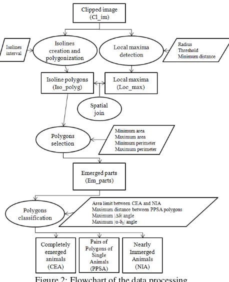
In order to facilitate the animal detection and counting, the selected images have been clipped to the portion containing hippos, surrounding areas being cut off. Those clipped images (Cl_im) are the starting point of the process. A flowchart of data processing is provided in Figure 2.
Figure 1: Graphical User Interface into QGIS for the specification of parameters and the presentation of results.
Figure 2: Flowchart of the data processing.
After georeferencing the image in a relative coordinate system (in pixel unit), the first step of the algorithm consists in detecting local maxima within the Cl_im, by using a fixed circular window. This part of the algorithm is adapted from FUSION tool developed by McGaughey et al. (2004). Those local maxima (Loc_max) are supposed to correspond to
centroids of emerged parts of animals. The search radius was fixed at 11 for the height of 39 meters and at 3 for the heights of 49, 73 and 91 meters. Indeed, this parameter can be adapted, depending on the resolution of the raster and the contrast among pixels values. The chosen value of this radius has to be a good compromise between the detection of all hippos and the avoidance of too many resulting points. A threshold raster value is also used in order to avoid the creation of points corresponding to water areas. This threshold was fixed at 100 for this research. In order to be sure that points correspond to different animals, a minimum distance between local maxima is also fixed. A value of 5 pixel units was retained.
Then, isolines were generated in order to connect pixels with the same raster value, considering a certain interval between contour values (we used an interval of 3). Closed isolines were then transformed into polygons (Iso_polyg).
Loc_max and Iso_polyg layers were then spatially joined, in order to link each local maximum to polygon containing it (n to n join).
The next step consists in selecting polygons that (i) contain at least one local maximum and (ii) whose area and perimeter are between minima (min_area, min_perim) and maxima (max_area, max_perim) values. Those four parameters were expressed as regression equations, as explained below.
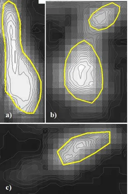
When several polygons contain the same Loc_max, only the largest one is kept for the next step. These polygons are supposed to correspond to emerged parts of animals (Em_parts). A single animal can have one or two emerged part(s). Globally, three cases can be distinguished on images: large polygons corresponding to completely emerged animals (CEA, Figure 3a), pairs of small to medium aligned and close polygons corresponding to a single animal (PPSA, Figure 3b), and small isolated polygons corresponding to nearly immerged animals (NIA, Figure 3c).
If a hippo is considered to be composed of two polygons, these two parts are supposed to be both close together, smaller than a completely emerged animal and have their main axis aligned. Polygons size, proximity and alignment criteria were applied to aggregate polygons pairs supposed to correspond to a unique hippo. Polygons size and proximity criteria were defined with regression equations presented below. For the alignment rule of polygons judged to be small, we have considered their relative orientation before merging them (Figure 4). It was necessary to build Minimum Bounding Boxes (MBB) around those small polygons to obtain their orientation characteristics. MBB are in this case the minimum enclosing rectangle for a polygon with the smallest area within which the entire polygon lies. Then, the criteria of position and alignment were built with the use of two angles. Firstly, the angle made by the longer axis of each polygon with the horizontal line was computed (ϑ0 and ϑ1 in Figure 4). The difference between those two angles constitutes the first angle parameter used in the algorithm: |Δϑ|. Secondly, the difference between two other angles is calculated (|α-ϑ0|): one is made by the line joining the centroids of the two polygons and the horizontal line (α in Figure 4), and the other corresponds to the angle of the longer axis of the first polygon with the horizontal line (ϑ0 in Figure 4). A maximal value of 30 degrees was considered for those two angular parameters.
As a result, the last part of the algorithm determines the number of animals represented by only one big polygon (CEA), the
number of hippos corresponding to paired polygons (PPSA), as well as the number of the other small isolated spots (only head or back above water, NIA).
Figure 3: a) Example of a completely emerged animal (CEA); b) Example of a pair of polygons corresponding to a single animal
(PPSA); Example of a nearly immerged animal (NIA).
Figure 4: Creation of Minimum Bounding Boxes (MBB) and representation of ϑ0, ϑ1 and α angles for the implementation of
alignment rule between PPSA polygons.
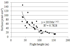
As mentioned above, six regression equations were computed and included in the algorithm in order to automatically estimate input parameters as a function of flight height. Data used for those regressions were based on the 37 images extracted from videos and the following manual digitization of 1856 hippos. In all, 32 different flight heights were represented among those 37 images. The first resulting models are polynomial and linear equations respectively for area and perimeter parameters (black curves in Figures 5 and 6). For each of those four datasets, the
32 values were divided in eight classes and the maximum (or minimum, according to the estimated parameter) value of area/perimeter was selected for each class to build four new regression equations (two polynomial and two linear ones again). Those four resulting equations (showed in red in Figures 5 and 6) were used to estimate the polygon selection parameters in the application, in order to extend the range of selectable polygons and taking variability of measures into account as far as possible. The set of 1856 digitized hippos was then used to model the relationship between flight height and the threshold area between NIA and CEA polygons (Figure 7). For each image, this threshold area was computed as the mean value of upper confidence bound of NIA polygons area and the lower confidence bound of CEA polygons area. The digitized hippos were also used to estimate the maximal distance between the two parts of PPSA according to flight height (Figure 8).
Figure 5: Polynomial regressions for the determination of maximal and minimal surfaces used in polygons selection. The
red curves represent the final equations used as input parameters in the algorithm.
Figure 6: Linear regressions for the determination of maximal and minimal perimeters used in polygons selection. The red lines represent the final equations used as input parameters in
the algorithm.
Figure 7: Polynomial regression of the evolution of threshold area between NIA and CEA polygons with flight height.
Figure 8: Linear regression between flight height and the maximal distance between centroids of two paired polygons
(PPSA).
3. RESULTS
The 4 images used to test the algorithm were acquired during the rainy season at altitudes ranging from 39 to 91 meters. At those altitudes, the estimated pixel ground sample distance is varying from 3.9 to 9.1 centimeters.
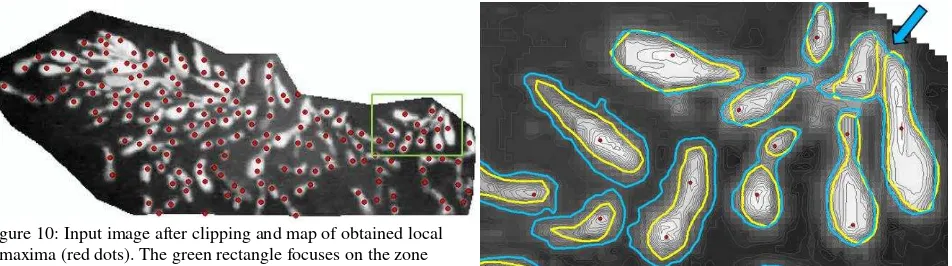
Several intermediate results of the processing are illustrated in Figures 9 to 12 for image coded 1_39_flight46 (codification present in Table 2). The four used images are provided in appendix. The sample image is interesting as it illustrates the necessity to mask areas corresponding to the riverbank. This image was taken at 39 meters above ground level at 12:26. Figure 9 corresponds to the original image whereas Figure 10 illustrates the clipping process and the generation of local maxima. Figure 11 shows local maxima and isolines, whereas Figure 12 contains manually digitized polygons and the polygons resulting from the automatic process with their corresponding local maxima.
Figure 9: Input image before clipping.
Figure 10: Input image after clipping and map of obtained local maxima (red dots). The green rectangle focuses on the zone
represented in Figures 11 and 12.
Figure 11: Local maxima (red dots) and isolines (in green) for the upper-right part of the input image.
Figure 12: Manually digitized polygons (yellow) and polygons generated and selected by the algorithm (blue) with
their corresponding local maxima (red). The blue arrow indicates an error of the automatic procedure, joining two close
hippos as a single one.
The total number of animals detected by the algorithm varies between 74 and 108 (Table 2). It shows a good agreement with reference values derived from manual counting: the error is ranging from -9.8% to +13.7%, with a mean value of +2.3%, which is not significantly different from 0 (p = 0.67). The correlation between total estimated and reference values reaches 0.86 (Table 3). If we analyse the distribution of counts among the different classes (Table 3), we can observe a good concordance (estimated vs observed) for NIA values (r = 0.93), whereas the situation is less favourable for both PPSA (r = 0.48, not significant) and CEA counts (r = -0.72).
Table 2: Comparison of manual and automatic counts of hippos on the four selected images: NIA (Nearly Immerged Animals), PPSA (Pairs of Polygons corresponding to Single Animals) and CEA (Completely Emerged Animals). Estimation errors are also provided.
Image code Height (m)
Manual count Automatic count Error
NIA PPSA CEA Total NIA PPSA CEA Total
1_39_flight46 39 34 44 27 105 37 15 56 108 +2.9%
2_49_flight53 49 24 10 48 82 22 18 34 74 -9.8%
3_73_flight53 73 24 8 41 73 27 3 53 83 +13.7%
4_91_flight53 91 33 6 47 86 33 6 49 88 +2.3%
Mean +2.3%
Table 3: Correlation coefficients (and associated p-values) between manual and automatic counts. NIA counts PPSA counts CEA counts Total counts Manual – automatic correlation 0.93 (p = 0.07) 0.48 (p = 0.52) -0.72 (p = 0.28) 0.86 (p = 0.14)
4. DISCUSSION AND PERSPECTIVES
4.1 Image processing
The comparison between visual and estimated counts showed very similar results for the set of test images (unbiased estimations with error ranging from -9.8% to +13.7%).
Few false positives local maxima were generated. But they were either contained in unselected polygons or not contained in any polygon, and thus they had no impact on the final estimation. The number of local maxima was strongly affected by the radius parameter. A high value minimizes the false positives but increases the risk of non detection of animals, especially the nearly immerged ones, which represent one third of the group. It is thus important to fix this parameter carefully.
The shape of selected polygons (Em_parts) can be rather different from that of manual delineations. Furthermore, some very close hippos were an important issue to deal with. The range of parameters values used in the polygons selection process did not always permit to distinguish efficiently those problematic cases (example in Figure 12).
Another weakness of the algorithm concerns the cases where the head of a hippo is not in the axis of its back (head turned on the side). Indeed, the relative alignment of neighbour polygons is involved in the aggregation rule. This criterion could be made more flexible, but false associations between shapes could become a more important source of error.
For NIA, manual and automatic counts seem to give really close results (Tables 2 and 3). It is different for PPSA and CEA and both visual and automatic procedures show uncertainties
identifying them. Nevertheless, those results tend to compensate and give a similar total headcount. Anyway, those assertions have to be confirmed by a test of the application on a larger dataset.
In each image, the group of hippos has to be manually bounded by drawing a mask around it. This step is really important to get valid results. Indeed, ground and vegetation around the pool have a high reflectance in thermal wavelength and appear bright. Therefore the value of those pixels could interfere with identification of hippos and lead to false detections. A perspective could be the automation of the masking process in order to reduce manual operations. This should be possible with the consideration of both the size of template objects and the reflectance variation around them.
The processing developed in this study does not use texture analysis or regular pattern recognition as other authors did (Laliberte & Ripple, 2003; Gougeon, 1995; Meyer et al., 1996; Quackenbush et al., 2000; Abd-Elrahman et al., 2005). Indeed, the provided images do not present enough texture variations compared to classical RGB images in high resolution. For the classification by pattern recognition, a major difficulty has to be taken into account: unlike animals in other studies, visible
4.2 Conditions of use of the algorithm
The very little difference between automatic and visual counts of hippos highlights the real interest and promising perspectives of the presented tools. But it now needs to be tested on a larger dataset corresponding to a wider range of conditions to confirm its real interest. Indeed, several limitations pointed out in the present study still have to be addressed.
Gathering of 10 to 200 individuals is frequent for this species (Delvingt, 1978). The images used in this study thus totally match with hippo’s natural behavior. As results show it, the application is adapted for high concentrations of animals but still has to be tested on a larger dataset with various headcounts.
According to the analysis of the whole set of thermal infrared data acquired above hippos during the two months in the field (September 2014 and May 2015), some practical implications can be proposed. We recommend doing flights during the rainy season (April to November) if possible. Indeed, large amount of chilly rainwater permits to get a better temperature contrast between hippos and their background during this period. We have also seen impacts of time of the day and weather on the visibility of hippos. However, our small dataset does not permit to determine the best combination of those factors for an optimal detection of hippos on infrared thermal imagery.
Manual contouring to compute surfaces and perimeters were used to reckon polygon sizes for each image out of the total of 37 acquired. The objective was to determine the sizes (in pixel unit) of the smallest and largest polygons as a base-line for the polygon selection in relation with height of the UAV. This calibration of input parameters was made in order to be flexible with flight altitude and permits to use images acquired from a large amplitude of heights, ranging from 38 to 155 meters. However, more robust regressions could be obtained with a
more restricted range of heights and could lead to more reliable counting results.
4.3 Exploitation of results
Unlike the main other studies relying on a similar procedure, numbers of animals in this case is low, generally in the range from 101 to 102. In comparison, other studies (Table 1) mainly focus on birds populations, dealing with headcounts sometimes reaching thousands of individuals. An error expressed in percent is then maybe not the best way to judge of the quality of this method in comparison with others if we talk about the accuracy in number of individuals.
Another thing to put in perspective is that the count itself is not completely representative of the real group size. Indeed, the algorithm processes single images giving instantaneous estimates in which only visible individuals at this moment are taken into account. As we have seen in the field, thermal infrared cameras are not able to detect heat sources under cover and even a thin water layer can hide animals. It thus does not allow us to determine the exact number of animals present within the area as it is a well-known fact that at least a fraction of hippos are fully under water (Delvingt, 1978). The calculation of a correction factor applied to the count from a single image could be realized to estimate the number of the entire population, including hippos under water. Delvingt (1978) has studied the diving rhythm of hippos to compute such a correction of counts and obtained a value of 1.25 in the case of Virunga National Park (DRC). This correction factor basis of one pixel size, it could be possible to measure animals’ backs. Such a quantification of lengths could lead to the creation of a histogram presenting the distribution of headcounts in each age classes.
4.4 Sensors and UAV improvement
To improve ground truth reference, a double payload could be used on the UAV. Indeed, thermal infrared and high resolution real colors images acquired simultaneously could permit a better interpretation of acquired images. However, the combination of those two types of sensors on the Falcon Unmanned UAV is not possible for the moment. An automatic procedure integrating visible and near infrared imagery with thermal infrared could also be valuable, but there is a need to match all of those data with accuracy, which is not yet possible with our current techniques. Some improvements in the use and exploitation of infrared images could help in building such processing, notably in the georeferencing step. For the detection of hippos in large areas, a combination of infrared videos and RGB digital camera could be a useful solution: Franke et al. (2012) tried with success to first detect animals on infrared videos and then identifying species (red deer, fallow deer, wild boar, roe deer, foxes, wolves and badgers) and numbers of individuals with high resolution real colors images acquired simultaneously. As well, the use of high resolution thermal infrared photos instead of videos in low quality would also be a substantial technical improvement.
Using a multicopter platform instead of a fixed wing UAV could also be a valuable solution for such a study. Actually, a multicopter would be useful to take advantage of a stationary position of the sensor in order to acquire a time series of images whose interest has been previously mentioned.
5. CONCLUSION
The development of UAV technologies for the monitoring of wildlife fauna will keep expanding during the coming years. The huge amount of data being one of the main drawbacks for the use of drones in natural resources management, the development of such algorithm is very important to create a viable monitoring system. Automation of image processing allows operators to save a lot of time, in particular for animal counts. Several notable advantages can be retained from this first algorithm attempting to automatically count hippos. First, the time spent by the operators to prepare and analyze the data is very reduced (limiting itself to the selection of images and to the manual demarcation of the group). The integration of the algorithm within a practical open source application with graphical interface to generate the resulting maps increases its added value as it is very easy to use and visualise. Furthermore, this method constitutes a standardized and reproducible procedure, avoiding the interference of a possible operator effect in the results. Finally, the parameters entered in the algorithm are modifiable to adapt to other situations or sensors. Indeed, all of those entry elements are defined by default but another sensor resolution could be used with a modification of local maxima entry parameters, just like polygons sizes if an operator would like to try an identification of hippos out of water during the night, for instance.
ACKNOWLEDGEMENTS
The authors would like to thank the European Union, the CIFOR (Center for International Forestry Research) and the Forest and Climate Change in Congo project (FCCC) as well as R&SD for granting and support this study. Special thanks also to the ICCN (Institut Congolais pour la Conservation de la Nature) and African Park Network teams involved in the protection and management of Garamba National Park for their help. Thanks to Laurent Dedry, Olivier De Thier, Adrien Michez and Sébastien Bauwens for some runways and ideas of research to develop this algorithm.
REFERENCES
Abd-Elrahman, A., Pearlstine, L. & Percival, F., 2005. Development of Pattern Recognition Algorithm for Automatic Bird Detection from Unmanned Aerial Vehicle Imagery.
Surveying and Land Information Science, 65(1), pp. 37–45.
Chabot, D., 2009. Systematic evaluation of a stock Unmanned Aerial Vehicle (UAV) system for small-scale wildlife survey applications. M.Sc. Thesis. McGill University, Montreal, Quebec, Canada.
Cunningham, D.J., Anderson, W.H. & Anthony, R.M., 1996. An image-processing program for automated counting. Wildlife Society Bulletin, 24(2), pp. 345-346.
Delvingt, W., 1978. Ecologie de l’hippopotame (Hippopotamus amphibius L.) au Parc National des Virunga (Zaïre). Thèse de doctorat. Faculté des Sciences Agronomiques de l’Etat, Gembloux, Belgique.
Franke, U., Goll, B., Hohmann, U. & Heurich, M., 2012. Aerial ungulate surveys with a combination of infrared and high-resolution natural colour images. Animal Biodiversity and
Conservation, 35(2), pp. 285-293.
Gilmer, D.S., Brass, J.A., Strong, L.L. & Card, D.H., 1988. Goose counts from aerial photographs using an optical digitizer.
Wildlife Society Bulletin, 16(1), pp. 204-206.
Gougeon, E.A., 1995. Comparison of possible multispectral classification schemes for tree crowns individually delineated on high spatial resolution MEIS images. Canadian Journal of
Remote Sensing, 21(1), pp. 1-9.
Grenzdörffer, G.J., 2013. UAS-based automatic bird count of a common gull colony. In: International Archives of the Photogrammetry, Remote Sensing and Spatial Information
Sciences, XL-1/W2(4-6 September), pp. 169–174.
Jones, G.P., Pearlstine, L.G. & Percival, H.F., 2006. An Assessment of Small Unmanned Aerial Vehicles for Wildlife Research. Wildlife Society Bulletin,34(3), pp. 750-758.
Koh, L.P. & Wich, S.A., 2012. Dawn of drone ecology: low-cost autonomous aerial vehicles for conservation. Tropical
Conservation Science, 5(2), pp. 121-132.
Laliberte, A.S. & Ripple, W.J., 2003. Automated wildlife counts from remotely sensed imagery. Wildlife Society Bulletin, 31(2), 362-371.
Linchant, J., Lejeune, P. & Vermeulen, C., 2014. Les drones au secours de la grande faune menacée de RDC. Parcs & Réserves, 69(3), pp. 5–13.
McGaughey, R.J., Carson, W.W., Reutebuch, S.E. & Andersen, H.E., 2004. Direct measurement of individual tree characteristics from LIDAR data. In: Proceedings of the Annual
ASPRS Conference, Denver, May 23-28, 2004. American
Society of Photogrammetry and Remote Sensing, Bethesda,
MD.
Meyer, P., Staenz, K. & Itten, K.I., 1996. Semi-automated procedures for tree species identification in high spatial resolution data from digitized colour infrared-aerial photography. ISPRS Journal of Photogrammetry and Remote Sensing, 51(1), pp. 5-16.
Mulero-Pázmány, M., Stolper, R., Van Essen, L.D., Negro, J.J. & Sassen, T., 2014. Remotely Piloted Aircraft Systems as a Rhinoceros Anti-Poaching Tool in Africa. PLoS One, 9(1), pp. 1-10.
Quackenbush, L.J., Hopkins, P.F. & Kinn, G.J., 2000. Developing forestry products from high resolution digital aerial imagery. Photogrammetric Engineering and Remote Sensing, 66(11), pp. 1337-1346.
Sasse, D.B., 2003. Job-related mortality of wildlife workers in the United States, 1937-2000. Wildlife Society Bulletin, 31(4), pp. 1000-1003.
Vermeulen, C., Lejeune, P., Lisein, J., Sawadogo, P. & Bouché, P., 2013. Unmanned Aerial Survey of Elephants. PLoS One
8(2), e54700.
APPENDIX
Image 1_39_flight46
Image 2_49_flight53
Image 3_73_flight53
Image 4_91_flight53