L
Journal of Experimental Marine Biology and Ecology 247 (2000) 243–255
www.elsevier.nl / locate / jembe
Hypoxic effects on growth of Palaemonetes vulgaris larvae
and other species:
Using constant exposure data to estimate cyclic exposure
response
a ,* b a
Laura L. Coiro , Sherry L. Poucher , Don C. Miller
a
U.S. Environmental Protection Agency, Atlantic Ecology Division, 27 Tarzwell Drive, Narragansett,
RI02882, USA
b
Science Applications International Corporation, 221 Third Street, Newport, RI 02840, USA Received 1 December 1999; received in revised form 18 December 1999; accepted 3 January 2000
Abstract
First stage larval marsh grass shrimp, Palaemonetes vulgaris, were exposed to patterns of diurnal, semidiurnal, and constant hypoxia to evaluate effects on growth and to determine if there was a consistent relationship between exposures. A comparison of growth with cyclic exposures versus constant low dissolved oxygen (D.O.) concentrations equivalent to the minima of the cycles showed the cyclic exposures resulted in less growth impairment than constant low-D.O. exposures, when compared to saturated controls. The mean extent of growth impairment of cyclic hypoxia was, however, almost 1.5 times more than would be estimated using an arithmetic time-weighted-average of the hypoxic portion of the cycle. Additional testing with other life stages and species resulted in similar patterns of response. Based on this relationship, an adjusted time-weighted-average could be used to estimate field related responses to cyclic dissolved oxygen from laboratory-derived constant exposure data. 2000 Elsevier Science B.V. All rights reserved.
Keywords: Cyclic exposure; Dyspanopeus sayi; Growth; Hypoxia; Marsh Grass Shrimp; Palaemonetes
vulgaris; Paralichthys dentatus; Say Mud Crab; Summer Flounder
1. Introduction
Dissolved oxygen (D.O.) conditions in aquatic systems are rarely stable. Episodes of low-D.O. are driven by biotic and abiotic factors such as photosynthesis and respiration,
*Corresponding author. Tel.:11-401-782-3000; fax:11-401-782-3030.
E-mail address: [email protected] (L.L. Coiro)
tidal cycles, and weather patterns. The variability associated with episodes of hypoxia (dissolved oxygen below air-saturation) is unique to each site and season. For example, in the northeastern United States, low dissolved oxygen can persist over much of the summer, as is often experienced in the waters of western Long Island Sound (Welsh et al., 1994), or can cycle daily with the tide, as is characteristic of Chesapeake Bay and its tributaries (Sanford et al., 1990; Diaz et al., 1992). How low-D.O. affects the biota of aquatic systems is related to duration and frequency as well as intensity of the event. Although hypoxic events can eventually lead to mortality, more commonly they lead to sublethal effects such as reduced growth, changed metabolism, and delayed develop-ment. Compared to conditions that cause mortality, sublethal levels of D.O. are generally less severe, longer-lasting and more widespread.
Research on the oxygen requirements of aquatic animals has focused primarily on the lethal and sublethal effects of continuous exposure to reduced oxygen. To better evaluate risk from intermittent or cyclic hypoxia, research is needed that reflects naturally occurring patterns of low dissolved oxygen. However, given the complexity of cyclic exposure testing, there has been little research addressing the effects of this phenom-enon. Because cyclic hypoxia is so variable, it is preferable to use a modeling approach to assess the possible effects on a system. In a system that experiences time-variable hypoxia, the degree to which an individual organism will be affected by low-D.O. induced stress may be best described by the cumulative effect of exposures over the annual growth period. The intent of this study was to establish a method for estimating the effects associated with multiple exposures to cyclic hypoxia using easily-derived constant-exposure growth data as the foundation. In laboratory tests, growth of an organism is often the sublethal endpoint used and has been shown to be a more sensitive indicator of low dissolved oxygen than survival (e.g., Morrison, 1971; U.S. EPA, 1986; Das and Stickle, 1993; Thursby et al., 1997). One model for estimating this cumulative effect would be to prorate known laboratory responses from constant-D.O. exposure testing to reflect the actual field exposure, but the accuracy of this approach has never been systematically tested. In application, having estimated response patterns which relate effects under non-constant conditions to known responses from constant exposure testing would allow for more meaningful assessments of risk, without requiring the difficulty of cyclic exposure testing.
In this study, we measured the growth of a larval estuarine crustacean, Palaemonetes
vulgaris in five tests involving both constant and fluctuating low-D.O. conditions. Tests
which support the findings of this study were also conducted with juvenile P. vulgaris, larval Say mud crab (Dyspanopeous sayi ), and juvenile summer flounder (Paralichthys
dentatus), but these results will not be discussed at length here because the data sets are
was expected, but the underestimation was fairly consistent and could therefore be adjusted to provide a reasonable estimate of effect which was still related to the time component of exposure.
2. Materials and methods
2.1. Animal culture
Adult marsh grass shrimp (Palaemonetes vulgaris) were collected from Narragansett Bay, RI, embayments and the nearby Pettasquamscutt River. Parental stocks were maintained in 76 l flow-through aquaria supplied with 258C filtered Narragansett Bay seawater at a salinity of 28–32‰. Individual gravid females were isolated in static, aerated 3.8 l jars of seawater that were renewed daily. Larvae were collected from the jars within 24 h of hatching and placed directly into the test system. Adults and newly-hatched larvae were fed Artemia salina nauplii (Great Salt LakeE, Aquafauna, Hawthorne, CA) daily during laboratory holding and culturing. Test larvae were fed ad libitum rations twice daily during exposure, generally at the beginning of each D.O. phase (Reference Artemia Cysts II and III, Brazilian brand; Bengtson et al., 1985). Animals were fed at the same times in the constant D.O. treatments as in the fluctuating treatments. Excess food was removed prior to each feeding.
Juvenile grass shrimp were cultured in the same manner as larvae, except that they were maintained in the aerated jars and observed daily until transition to the first juvenile stage. Adult Say mud crabs were collected from Narragansett Bay and Pettasquamscutt River. Maintenance of parental stocks and rearing of larvae were similar to grass shrimp except that the larvae were removed from the jar after hatching and held in flow through mesh containers until used in the test. Post-metamorphosed summer flounder were obtained from the University of Rhode Island Graduate School of Oceanography (courtesy of D. Bengtson, Narragansett, RI). Prior to testing the fish were maintained in 76 l flow-through aquaria and were fed Artemia salina nauplii (Great Salt LakeE, Aquafauna, Hawthorne, CA) supplemented with flake fish food (TetraE SM80, Tetra Werke Baensch, Melle, Germany) daily during laboratory holding. During testing, the fish were fed ad libitum rations twice daily during exposure, (Reference Artemia Cysts II and III, Brazilian brand; Bengtson et al., 1985). Each feeding was supplemented with frozen adult Artemia salina (Pro SaltE, Mid Jersey Pet Supply, Carteret, NJ)
2.2. Low-D.O. test system
Treatment water was gravity-fed directly from mixing boxes to 500 ml exposure chambers at a rate of about 100 mls / min. Outflows from each chamber passed through a
10 cm circular Nytex screen (220 mm mesh) inserted in the lid. Each chamber was submerged in a 7 l aquarium with a glass cover to minimize the possibility of reaeration. Low-D.O. water was produced by vacuum-degassing. CO was bubbled back into the2 degassed water to restore and maintain a consistent pH of 7.8–8.2. Temperature was controlled electronically to 618C. Test salinity was ambient Narragansett Bay salinity, ranging from 28 to 32 l. The light cycle was 12 h light:12 h dark.
2.3. Test design and implementation
Tests usually consisted of four to six treatment concentrations and an air-saturated control. All low-D.O. concentrations were selected to be largely sublethal, as determined by previous constant exposure testing. There were four replicates per exposure, with ten to twenty animals per replicate. The test duration was four, seven, or eight days. Dissolved oxygen concentrations in the fluctuating exposures were continuously monitored in the chamber with a Nester oxygen meter (model 8500; BOD probes) and a chart recorder (Chino Corp. AH-11E Hybrid). Constant-exposure low-D.O. treatments, included for internal comparison, were checked with a Nester meter at least daily. Meters were calibrated daily with a modified Winkler method using saturated sea water. D.O. concentrations were checked against modified Winkler titrations at the beginning and end of each test. Salinity, temperature, and survival were also monitored daily.
This study used square-wave D.O. cycles since the results from these exposures are easier to interpret than continuously changing conditions, such as sine-wave cycles. The cycles had equal time at low-D.O. and saturated conditions. The cycles were 6 h low:6 h high or 12 h low:12 h high, with minimal transition times (Table 1). These conditions were chosen to represent semidiurnal and diurnal tidal cycles of hypoxia. All semidiur-nal treatments started with the maximum D.O. concentration in the early morning. In this regime, the light cycle began with the morning high-oxygen cycle. For diurnal cycles, the light cycle began 6 h after the start of the low-D.O. phase. The onset of the light cycle in the diurnal D.O. cycles was shifted so both cycle regimes had a period of light and dark during each phase (i.e. low-D.O. and saturation) of the cycle.
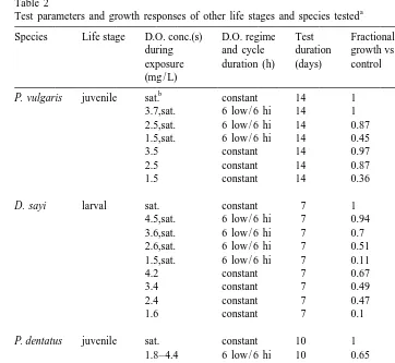
The methods used for the tests with juvenile P. vulgaris and other species were similar to the larval P. vulgaris tests, with modifications to the exposure chambers and test duration (Table 2). These tests only considered semidiurnal cycles and constant exposures. The exposure chambers for larval D. sayi and juvenile P. dentatus consisted of up to twelve individual 150 ml cups attached to a common baffle for each replicate. For P. dentatus each cup held an individual animal in order to follow the growth of that specific individual.
2.4. Growth endpoint
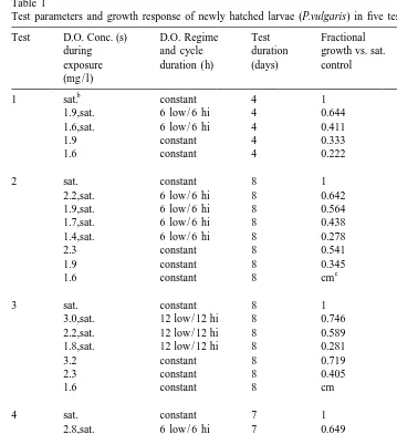
Table 1
a
Test parameters and growth response of newly hatched larvae (P.vulgaris) in five tests
Test D.O. Conc. (s) D.O. Regime Test Fractional Fractional
during and cycle duration growth vs. sat. difference from
exposure duration (h) (days) control sat. control
(mg / l)
Fractional growth (FG) calculated using Eq. (2). Difference from control calculated as (12FG). All treatments were significantly different from controls for each test (Duncan’s Multiple Range Test).
b
Air saturated.
c
Complete mortality.
— —
G5 3dry weight / animalfinal2 3dry weight / animalinitial (1)
Table 2
a
Test parameters and growth responses of other life stages and species tested
Species Life stage D.O. conc.(s) D.O. regime Test Fractional Fractional during and cycle duration growth vs. sat. difference from exposure duration (h) (days) control sat. control (mg / L)
b
P. vulgaris juvenile sat. constant 14 1 0
3.7,sat. 6 low / 6 hi 14 1 0
P. dentatus juvenile sat. constant 10 1 0
1.8–4.4 6 low / 6 hi 10 0.65 0.35
4.4 constant 10 0.89 0.11
1.8 constant 10 0.55 0.45
P. dentatus juvenile sat. constant 14 1 0
2.2,sat. 6 low / 6 hi 14 0.82 0.18
1.8,sat. 6 low / 6 hi 14 0.69 0.31
2.3 constant 14 0.67 0.33
1.8 constant 14 0.53 0.47
a
Fractional growth calculated using Eq. (2). Difference from control calculated as (12FG).
b
Air saturated.
calculated for each individual. The mean fractional growth (FG) (Tables 1 and 2) for each treatment was calculated as:
— —
FG5 3growthtreatment/3growthcontrol (2)
Time-weighted averaging was used to estimate responses to the cyclic exposures, based on responses to constant exposures. The FGtime-weighted average ( TWA) is the arithmetic mean of constant exposure responses at the maximum and minimum D.O. of the cycle weighted by exposure duration using the equation:
*
FGTWA5(FGmax D.O.% exposure timemax D.O.) *
where FGmax D.O. is the fractional growth of the constant exposure which corresponds to the high D.O. concentration of the fluctuation, FGmin D.O. is the fractional growth of the constant exposure which corresponds to the low-D.O. concentration of the fluctuation, and % exposure time is the portion of the whole cycle duration spent at each condition. In this study, the cyclic exposure time was 50%:50% which results in an estimate equivalent to 50% of the adverse effects observed in the continuous low-D.O exposure.
3. Results
In each of the five tests with larval P. vulgaris, each low-D.O.treatment, whether fluctuating or constant, reduced growth significantly relative to the saturated-D.O. control (P,0.003 – Duncan’s Multiple Range Test) (Table 1). At the lowest D.O. exposures in both the constant and fluctuating treatments (1.6 and 1.4 mg / l), growth rates were only 22% and 28% of the controls, respectively. Even at the highest hypoxic D.O. levels tested (3.4 and 3.2 mg / l), the growth rates were only 79–85% of the saturated controls.
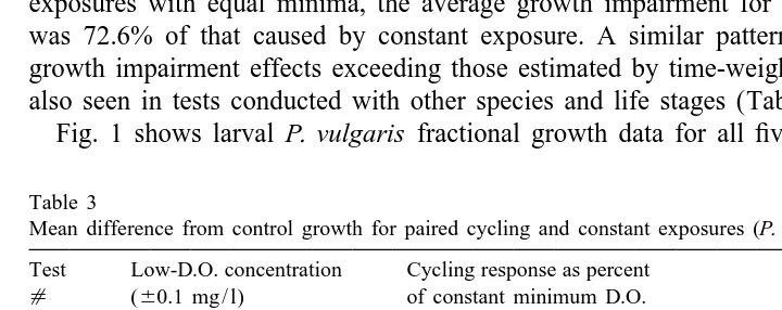
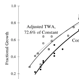
The results of the five independent sets of exposures were considered jointly to provide a general evaluation. Analysis of covariance showed that there was a significant difference (P,0.02) in growth impairment between cyclic exposures and constant low-D.O. exposures. Cyclic exposures usually resulted in better growth than corre-sponding constant exposures at D.O. concentrations equal to the minimum of the cycle. In comparison with the constant exposures, mean growth effects in the cyclic exposures ranged from 53 to 93% of the corresponding reduced growth of the constant low-D.O. exposure for paired data (Table 3). Considering all pairs of constant and cyclic exposures with equal minima, the average growth impairment for the cyclic exposure was 72.6% of that caused by constant exposure. A similar pattern of response, with growth impairment effects exceeding those estimated by time-weighted averaging, was also seen in tests conducted with other species and life stages (Tables 2 and 4).
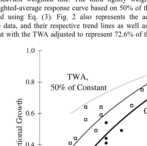
Fig. 1 shows larval P. vulgaris fractional growth data for all five sets of exposures
Table 3
Mean difference from control growth for paired cycling and constant exposures (P. vulgaris larvae) Test Low-D.O. concentration Cycling response as percent
Table 4
Mean difference from control growth of tested species for paired fluctuating and constant exposures, using pooled test results. Exposures considered paired if concentration is60.2 mg / l. D.O. of constant exposure (60.1 mg / l D.O.for P. vulgaris larvae)
Species Life stage Cyclic response Number of
as percent tests
constant response
Palaemonetes vulgaris larval 72.6% 5
Palaemonetes vulgaris juvenile 63.0% 1
Dyspanopeous sayi larval 83.3% 1
Paralichthys dentatus juvenile 61.0% 2
plotted against D.O. concentration. The fluctuating and constant exposure data have been
2 2
marked with best fit logarithmic trend lines (R 50.765 and R 50.945, respectively), the fluctuating exposure represented by the medium weighted line and the constant exposure by the heaviest weighted line. The third lightly weighted trend line represents the time-weighted-average response curve based on 50% of the constant exposure response, calculated using Eq. (3). Fig. 2 also represents the actual fluctuating and constant exposure data, and their respective trend lines as well as the estimated TWA response curve, but with the TWA adjusted to represent 72.6% of the constant exposure response,
Fig. 2. Actual fluctuating (h) and constant (d) growth response and adjusted estimated TWA response based
on 72.6% of the constant, as calculated using Eq. (3).
based on the results from these tests, which more closely represents the actual fluctuating response.
4. Discussion
consistent relationship is established, then continuous-exposure data could be used to estimate effects in natural systems experiencing fluctuating D.O.
There are likely several approaches that can be considered when trying to estimate effects of non-constant hypoxia using laboratory-derived continuous-exposure data. Two of the simplest are as follows. The first approach is to assume that the effect of a persistent cyclic exposure is the same as a constant exposure to hypoxic conditions of equal total duration. For example, a diurnal cycle of 12 h at high-D.O. and 12 h at low-D.O. would be assessed as if it had been a 24 h low-D.O. exposure. This approach only applies to the minimum concentration and therefore it is likely this would overestimate the response. The second option is to use a time-weighted approach where the estimated fluctuating effect is related in a time-proportioned manner to the actual duration of hypoxia during the cycle. Time-weighted averaging assumes nonlethal effects, such as reduced growth, are synchronous with the stress and do not extend beyond the period of exposure. While time-weighting may seem to be an appropriate approach to relate intermittent exposure to continuous hypoxia, and would provide a method to generalize for all types of exposures, this study has demonstrated that it underestimates actual growth reduction, at least for diurnal and semidiurnal cycles.
For the cyclic durations and D.O. exposures used in the tests presented here, the TWA estimated growth impairment under fluctuating D.O. conditions would be 50% of that under constant low-D.O. conditions. Yet, the observed effect of cyclic hypoxia with larval P. vulgaris was closer to 73% of the constant response. In work with freshwater juvenile largemouth bass, Stewart et al. (1967) saw a similar response pattern with cyclic hypoxia. In their experiment, the fish in the cyclic treatments were exposed to low-D.O. for eight or 16 h of the day. Under those conditions, growth impairment was almost always more than would have been estimated had the animals been held continuously at a concentration equal to the mean of the fluctuating exposure. Stewart’s data were reanalyzed using the TWA method to see if the results corresponded with those seen here when assessed in a similar manner. Using our method, growth impairment was usually more severe than the estimated TWA. Growth impairment greater than expected at the mean concentration of the fluctuation was also seen by Whitworth (1968) with brook trout and by Fisher (1963) with underyearling coho salmon. Revaluation of Fisher’s results again showed growth impairment that was more severe than the estimated TWA.
Why did the diurnal and semidiurnal cycles used in the tests presented here result in growth impairment that was almost 1.5 times greater than the TWA? A plausible explanation may be that the recovery following exposure to stress should not be expected to be instantaneous, but that hypoxia continues to affect the organism for a period after the D.O. returns to saturation, resulting in a lag in recovery.
Since there are numerous factors which may be influencing an animal’s ability to recover from low-D.O. stress, determining the major influences would allow for a more accurate application of TWA in estimating responses associated with natural fluctuating exposures. Little data exists on the factors associated with fluctuating D.O. which exert the strongest influences on this response. Factors which should be evaluated include the absolute degree of change in D.O., the slope of the transition between the minimum and maximum concentrations of exposure, duration of hypoxia within each cycle, and the amount of time at no-effect conditions between hypoxic periods of exposure. There are several possibilities for how these factors could influence growth-related recovery. The data from this study shows that over the entire sublethal D.O. range for growth of larval
P. vulgaris (1.4–3.2 mg / l) there was almost always more severe growth impairment associated with cyclic exposure as compared to the time-weighted response. This suggests that the absolute change in D.O., (i.e., amplitude of the cycle), may not be the most critical factor affecting subsequent recovery and growth. This study did not, however, address many of the other possible influences on D.O. exposure and recovery. For example, gradual changes in D.O., or other coexisting abiotic factors, may permit acclimation, resulting in incremental changes to respiration rate, feeding behavior, and metabolic activities which, in turn, may reduce impairment effects and allow quicker recovery. This was demonstrated by Cech et al. (1990), showing a relationship between temperature acclimation and changes in metabolic rates as they related to hypoxia. In general, those animals that were acclimated to temperature before experiencing hypoxic conditions had fewer significant changes in metabolic rates compared with those that experienced an abrupt temperature change immediately before hypoxic exposure.
The influence of duration of exposure and amount of time at non-stress conditions can affect recovery in many ways. One possibility is that there is a proportional relationship between the length of exposure and the amount of time needed to reach complete recovery and return to a normal growth rate. Another is that once the no-effect threshold has been exceeded, there is a discrete amount of time needed for recovery regardless of exposure duration.
All of the fluctuating exposures in this study had equal time under hypoxic and saturated conditions (50%:50%) and therefore only partially address the issue of the proportional relationship between exposure duration and recovery time. For larval P.
vulgaris, when there are equally proportionate exposure and recovery durations, growth
is impaired by nearly 1.5 times the expected amount. The two cycle durations (6 h low:6 h high or 12 h low:12 h high) and the different lengths of the tests (4 days, 7 days, or 8 days) did not appear to influence growth differently, possibly since the ratio of hypoxic exposure to saturated exposure is the same in all treatments, although there were not sufficient data to establish this point statistically. To better address which parameters are influencing recovery, additional testing with cycles of different regimes is required to determine the shape of the recovery curve for diurnal or semidiurnal patterns, as well as other patterns of fluctuation.
by a fairly consistent amount. The results presented here for P. vulgaris larvae and juveniles, D. sayi larvae, and juvenile P. dentatus, along with the work of Stewart et al. (1967), Whitworth (1968) and Fisher (1963), suggests that this pattern of enhanced growth impairment may occur in fishes as well as crustaceans. If the observed relationship between constant low-D.O. exposure response and fluctuating exposure response remains consistent across additional species, it will be reasonable to use an adjusted time-weighted average to assess potential hypoxia-induced stress on the biota in ecosystems experiencing diurnal and semidiurnal cycles.
5. Disclaimer
Mention of trade names or commercial products does not constitute endorsement or recommendation for use.
Acknowledgements
Portions of this work were sponsored by the U.S. Environmental Protection Agency under Contract 68-C1-0005 to Science Applications International Corporation. This paper is U.S. EPA Atlantic Ecology Division contribution number NHEERL-NAR 2066. The authors would like to thank the reviewers and other colleagues for their valuable input and they would like to acknowledge the laboratory efforts of Steve Rego, Nan Hayden, and Kathy Simmonin. [SS]
References
Bengtson, D.A., Beck, A.D., Simpson, D.L., 1985. Standardization of the nutrition of fish in aquatic toxicological testing. In: Cowey, C.B., Mackie, A.M., Bell, J.G. (Eds.), Nutrition and Feeding in Fish, Academic Press, London, pp. 431–435.
Cech, J.J., Mitchell, S.J., Castleberry, D.T., McEnroe, M., 1990. Distribution of California stream fishes: influence of environmental temperature and hypoxia. Environ. Biol. Fish. 29, 95–105.
Das, T., Stickle, W.B., 1993. Sensitivity of crabs Callinectes sapidus and C. similis and the gastropod
Stramonita haemastoma to hypoxia and anoxia. Mar. Ecol. Prog. Ser. 98, 263–274.
Diaz, R.J., Neubauer, R.J., Schaffner, L.C., Pihl, L., Baden, S.P., 1992. Continuous monitoring of dissolved oxygen in an estuary experiencing periodic hypoxia and the effect of hypoxia on macrobenthos and fish. Sci. Total Environ. Supplement, 1055–1068.
Fisher, R.J., 1963. Influence of oxygen concentration and of its diurnal fluctuations on the growth of juvenile coho salmon. M.S. Thesis, Oregon State Univ., Corvallis.
Miller, D.C., Body, D.E., Sinnett, J.C., Poucher, S.L., Sewall, J., Sleczkowski, D.J., 1994. A reduced dissolved oxygen test system for marine organisms. Aquaculture 123 (1994), 167–171.
Morrison, G., 1971. Dissolved oxygen requirements for embryonic and larval development of the hardshell clam, Mercenaria mercenaria. J. Fish. Res. Bd. Can. 28, 379–381.
Sanford, L.P., Sellner, D.R., Breitburg, D.L., 1990. Covariability of dissolved oxygen with physical processes in the summertime Chesapeake Bay. J. Mar. Res. 48, 567–590.
Thursby, G., Miller, D.C., Poucher, S., Coiro, L., Munns, Jr.,W.R., Gleason, T., 1997. Protection of Coastal and Estuarine Animals from Low Dissolved Oxygen: Cape Cod to Cape Hatteras. Submitted to U.S. Environmental Protection Agency, Office of Water, Office of Science and Technology, Washington, D.C. Contribution no. 1920.
U.S. EPA, 1986. Ambient water quality criteria for dissolved oxygen. U.S. Environmental Protection Agency, Office of Water Regulations and Standards. Criteria and Standards Division. Washington, D.C. EPA 440 / 5-86-003.
Welsh, B.L., Welsh, R.J., DiGiacomo-Cohen, M.L., 1994. Quantifying hypoxia and anoxia in Long Island Sound. In: Dyer, K.R., Orth, R.J. (Eds.), Changes in Fluxes in Estuaries: Implications from Science to Management, Olsen and Olsen, Fredensborg, Denmark, pp. 131–137.