The Effect of the 2007 Financial Crisis on the Asean Stock Indices’
Movements
Adwin Surja Atmadja
Faculty of Economics, Petra Christian University E-mail: [email protected]
ABSTRACT
This study attempts to examine the existence of cointegration relationship and the short run dynamic interaction among the five ASEAN stock market indices in the period of before and during the 2007 financial crisis. The multivariate time series analysis frameworks are employed to the series in both sub-sample periods in order to answer the hypotheses.The study finds two cointegrating vectors in the series before the financial crisis period, however it fails to detect any cointegrating vector in the period of financial crisis. Granger causality tests applied to the series reveal that number of significant causal linkages between two variables increase during the crisis period. Moreover, the accounting innovation analysis shows an increase in the explanatory power of an endogenous variable to another within the system during the crisis period, indicating that the contagious effect of the 2007-US financial crisis has entered into the ASEAN capital market, and significantly influenced the regional indices’ movements.
Keywords: ASEAN, stock market integration, the 2007 financial crisis, regional indices’ movements.
INTRODUCTION
Liberalization of the five ASEAN (Indonesia, Malaysia, the Philippines, Singapore, and Thailand) financial markets in 1980s resulted in enormous capital inflows to this region. By opening their national borders for foreign investors, the countries’ financial markets were overwhelmed by foreign capital in both foreign direct and portfolio investments giving significant support to their rapid domestic economic development, as well as enjoyed rapid financial markets expansion in the beginning of 1990s. Capital inflows have been crucial to the rapid - sustained growth in ASEAN countries (Sachs and Larrain, 1993:577) at that time, since domestic saving, as commonly in developing countries, had little role as development funding.
Triggered by the sharp depreciation of the Thai baht in the midst of 1997, the disastrous effects of the 1997 financial crisis were broadly spread out to the countries’ financial markets which were dominated by bank loan and portfolio investment, not by foreign direct investment (DFAT, 1999:29). The crisis then extensively affected the world financial markets through its contagion effects. Market capitalization of the countries’ stock market was largely contracted due to a deep depreciation in their stock prices causing their stock indices then sharply plunged.
However, the downturn in the five ASEAN rebounded in 1999. After the sharp output contraction in 1998, growth returned in that year as depreciated currencies spurred higher exports (Krugman and Obstfeld, 2003:693). Following the appreciation of regional currencies in the second semester of the year, the regional capital and financial markets started to recover. The regional stock market indices increased around 42.46% on average compared to those from two years before (calculated from IFS 2004). This might indicate that investors’ confidence started to recover and they began to invest in the five ASEAN.
During ten years after, the ASEAN’s economies steadily grew to their new equilibrium. As a market indicator, the ASEAN capital market indices apparently fluctuated in a relatively narrow range dominantly due to small internal shocks in the short run, but stably moved with positive trends in the long run. These all mirror that the ASEAN markets were relatively stable during the time periods, and their economies were just on the right tracks.
However, in the second semester of 2007 the countries experienced significant shocks in their capital markets due to a contagious effect of the US financial market turmoil. At the time, the US financial market deeply suffered from the most
significant economic shocks initiated by the sub-prime mortgage crisis leading to the downturn in housing market, and then worsened by the spike in commodity prices (Yellen 2008:1). The devastating effects of the 2007 financial crisis in the US then widely spread throughout the world.
From the facts above, the 2007 financial crisis may have significant consequences on the variation of the countries’ stock indices that probably different with those in non crisis era. The financial crisis could possibly cause the regional indices deviate from their long run equilibrium, and the behaviour of the indices’ movements may be different with those before. All possibilities may happen in the regional market depended on how significant the impact of the financial crisis hit the market. Therefore, this study will empirically examine how the 2007 financial crisis has taken into effect on the five ASEAN stock indices’ movements. To be more specific, this study attempts to observe the existing of cointegrating relationships among the five ASEAN stock indices in the periods of before (pre) and during the 2007 financial crisis in order to portray the long run interrelations among the indices in the both periods. The aim is also to answer how and to what extent the stock indices dynamically interact with each other in the short run during the given periods.
CONCEPT OF FINANCIAL MARKET OR STOCK MARKET INTEGRATION
The basic theoretical concept of financial market or stock market integration is adopted from the law of one price. In integrated financial markets, the assets with the same risk in different markets will result in the same yield when measured in a common currency (Stulz 1981:924-5). However, if the yields are different across the markets, the arbitrage process will play an important role in eliminating the differences. Operationally capital markets integration refers to the extent that markets’ participants are enabled and obligated to take notice of events occurring in other markets by using all available information and opportunities, while financial market integration is defined in terms of price interdependence between markets (Kenen 1976:9). Moreover, stock market integration is affected by some factors (Roca 2000:14), such as:
1. Economic integration, which means that the more integrated the economies of countries, the more integrated their equity markets (Eun and Shim 1989: 256).
2. Multiple listing of stocks. This implies that a shock in a particular stock market can be
transmitted to other stock market through shares listed in both markets.
3. Regulatory and information barriers. The higher the barriers, the lower the degree of stock market integration.
4. Institutionalisation and securitisation. As institutions are more willing to transfer funds overseas to increase their diversification opportunities, the integration will be promoted. 5. Market contagion. The prices between stock
markets can move together due to a contagion effect (King and Wadwhani 1990:5), and this contagion effect determines significantly the dynamic relationships between international stock markets (Climent and Meneu, 2003:111). However, in emerging stock markets, this effect might be smaller than what is widely perceived (Pretorius 2002:103).
Much research has been done, mainly by using a cointegration analytical framework, to find and analyse the existence of integration in stock market across countries. The results are different depending on where, when, and how the research has being conducted. The cointegration analytical framework has been widely applied to examine the integration of stock markets across countries. Once a cointegration vector is found among two or more stock markets, it indicates the existence of a long run relationship among them. Thus, stock price movements in one equity market will affect another in other markets.
A research conducted by Chung and Liu (1994:55) found two cointegration vectors between the U.S and larger Asia Pacific stock markets. Palac-McMiken (1997:299) also reveals the existence of cointegration in ASEAN markets (Malaysia, Singapore, Thailand, and the Philippines), except Indonesia, during 1987 to 1995. Both results were confirmed by Masih and Masih (1999:275) who report that some of ASEAN countries (Thailand, Malaysia, and Singapore) have a high degree of interdependence with other Asian (Hong Kong and Japan) and developed (the U.S. and the U.K.) stock markets. Furthermore, they also find one cointegration vector among several major Asian stock markets (Hong Kong, Korea, Singapore, and Taiwan) and major developed markets (Masih and Masih 2001: 580-1).
interdependency among all the ASEAN stock markets in the short run. However, in contrast to short run interdependency, he indicates that there was no cointegration among ASEAN countries as a group during 1988-1995 and that those stock markets were not significantly related to each other in the long run.
Chan, Gup and Pan (1992:289) and DeFusco, Geppert and Tsetsekos (1996:343) also mention that there is no cointegration between the U.S and several Asian emerging stock markets (Hong Kong, Taiwan, Singapore, Korea, Malaysia, Thailand, and the Philippines) in the 1980s and early 1990s. However, these findings somewhat contradicts with those of Chung et al. (1994) and Masih et al. (1999). This then implies that the interdependence among stock markets is not stable over time. For example, Hung and Cheung (1995:286) assert that there is no cointegration among stock markets in some Asia-Pacific countries (Malaysia, Hong Kong, Korea, Singapore, and Taiwan). However, when they used US dollar denominated stock prices, it was reported that those stock markets were cointegrated after, but not before, the 1987 stock crash.
Arshanapalli and Doukas (1993:206) also mention the instability of stock market interdependence when they tested the effect of inclusion or omission of the data for the 1987 crisis and revealed that that it affects the results. They conclude that the stock markets were highly integrated during the crisis. Furthermore, Arshanapalli, Doukas and Lang (1995:72) show that after the 1987 crisis the stock markets in emerging markets (Malaysia, the Philippines, and Thailand) and developed markets (Hong Kong, Singapore, the U.S., and Japan) are more interdependent as they found cointegration in the post-crisis period, but not in the pre-crisis period. Other researchers, Liu, Pan and Shieh (1998: 59) also confirm that there is an increase in the interdependence within Asian-Pacific regional markets and the stock markets in general post-the 1987 crisis. Similarly, Sheng and Tu (2000:245) document one cointegration vector between the U.S. and several Asian stock markets (Taiwan, Malaysia, China, Thailand, Indonesia, South Korea, the Philippines, Australia, Japan, Hong Kong, and Singapore) during the crisis, but none in the year before the crisis, when they observed the stock markets using daily data.
Finally, a research recently conducted by Yang, Kolari and Min (2003:478) examined the long-run relationship and short-run dynamic causal linkages among the U.S, Japanese, and ten Asian emerging markets using daily data of 1997-1998 periods. They confirm that the stock markets
of those countries have been more integrated after the 1997 Asian financial crisis than before the crisis. Both long-run cointegration relationship and short-run causal linkages among those markets become more significant during the crisis. These findings also confirm that the degree of integration among those countries tends to change over time.
Several points that may be drawn form the literature review. The implication is that liberalization of the financial sector in many countries has caused world or regional stock markets to be more integrated. Empirical evidence is given by the presence of cointegration vectors and significant short-run causal linkages. It is worth noting that the stock markets of countries in the same region may be more interdependent than those in different regions.
RESEARCH METHODOLOGY
Basically, a stock market price index or stock market index is a portfolio of individual stocks. The index level corresponds to some average of the price levels of individual shares. Changes in the index level give rise to market returns. Thus, the stock market index, which can be viewed simply as a portfolio of shares, can commonly be use as an indicator of the market performance. There are several factors that determine the level of the index, such as breadth of index, weighting system, capitalization adjustment, and dividend effect (Brailsford Heaney and Bilson 2004:68).
The stock market index of a country may also be an indicator of short-term portfolio investment movement in the country. An upward trend of a stock market index means that there is an increase in demand of the listed shares in the market. This indicated that investors are attracted to buy shares and invest their fund in the country. On the other hand, a downward trend movement of a stock market index indicates that the investors are unlikely to continuously hold the listed shares. Hence, stock market movements may reflect the attractiveness of a country for investments, especially for portfolio investments.
In this study, the daily closing stock price indices of the five ASEAN countries, which are Jakcomp of Indonesia; KLSE of Malaysia; PSEi of the Philippines; STI of Singapore; and SET Composite of Thailand, are employed as measurement of the countries’ daily stock index movements in the periods of before and during the 2007 financial crisis.
region are interdependent not only among themselves, but also with some of the developed market. Furthermore, those stock markets are even more interdependent during and after the financial crisis (Sheng et al 2000; Yang et al 2003)
In the case of the ASEAN, Palac-McMiken (1997:299) reports the existence of cointegration in the countries’ stock markets, except Indonesia, before the 1997 crisis. Yang et al (2003:478) confirm that both long-run cointegration relationship and short-run causal linkages among those markets become more significant during the crisis period. In contrast, Roca (2000:145) finds the existence of interdependency among the five ASEAN’s stock markets in the short run, but not significantly related in the long run before the 1997 crisis.
Based on these findings, it is hypothesized that the ASEAN stock indices would have long run cointegration relationship and short run dynamic interaction, and that the relationship and the interaction would be more significant during the 2007 financial crisis.
All daily price index data of the five ASEAN during the observation periods are obtained from the Thomson Financial. The index data of all variables then will be transformed into natural logarithm forms before conducting the analyses.
In order to examine the movements of the indices in both periods, the data are then separated into two sub-sample periods, which are the periods of: 1) Before the 2007 financial crisis (pre crisis), which cover the period of Jan 2000 – June 2007, 2) During the 2007 financial crisis, which cover the period of July 2007 – May 2009, as it is stated in several publications (http://en.wikipedia.org,www. globalissues.org,www.atypon-link.com)
The two most appropriate models that one of which may suitable for this study are VAR and VECM. In the Vector autoregressive model (VAR) all of the variables are endogenous, and symmetrically treated. A VAR could be very large, however the simplest VAR model, in standard form, could be written as (Enders, 2004:265): Yt = a10 + a11Yt-1 + a12 Zt-1 + eYt.
Zt = a20 + a21Yt-1 + a22 Zt-1 + εZt.
The VAR requires that all variables be stationary and the appropriate lag length is data driven (Brooks 2002:333). There are several available tests for testing for a unit root, the most common is the Augmented Dicky-Fuller (ADF) test. Non-stationary variables may be made stationary by differencing or detrending process.
To define the appropriate lag length, some tests of information criteria that will be applied in this study include the likelihood ratio test; Akaike
Information Criterion (AIC); and Schwarz Bayesian Criterion (SC).
The likelihood ratio test is based on asymptotic theory and is an F-type approximation. This test actually compares a restricted VAR (less lags) to an unrestricted VAR (more lags). Thus, the null hypothesis of this test is that the restricted model is correct. However, the shortcoming of this test is that it may not be useful in small samples. In addition, the likelihood ratio test is only valid when the restricted model is tested (Enders 2004:283).
Because of the limitations of the likelihood ratio test, multivariate generalization of AIC and SC may be the most suitable alternatives. The minimum values of AIC and/or SC may validly indicate the appropriate lags length, as long as the model’s residual has no serial correlation problem. Otherwise, the lag length may be too short. Thus, it is necessary to re-estimate the model using lag length that yield serially uncorrelated (Enders 2004:338).
In VAR, a block causality test will be used to examine whether the lags of one variable enter into the equation for another variable (Enders 2004:283). A variable (y1) is said to be a
granger-cause of another (y2) if the present value of y2 can
be predicted with greater accuracy by using past values of y1, all other information being identical
(Thomas 1997:461). If y1 granger-causes y2, then
the parameters of lags of y1, βi’s, should not equal
zero in the equation of y2. However, it is worth
noting that granger-causality basically means a correlation between the current value of one variable and the past (lags) value of others. It does not mean that movements of one variable physically cause movements of another (Brooks, 2002:240). Granger causality simply implies a chronological ordering of movements of the series. Therefore, it could validly be stated that changes or movements in one variable (y2) appear to lag those
of another (y1).
The alternative model that probably suitable to be used is the vector error correction model (VECM) or cointegration framework analysis, which is basically is a VAR augmented by the error correction term (êt-1). The simplest VECM, in
general, takes the form as (Enders 2004:329):
ΔYt = α10 + αY êt-1+ ∑α11(i) ΔYt-i + ∑α12(i) ΔZt-i + εYt. ΔZt = α20 + αZ êt-1+ ∑α21(i) ΔYt-i + ∑α22(i) ΔZt-i + εYt.
where
êt-1 = (Yt-1 – β1Z1t-1)
Thus, if the parameters of error correction term (ECT), called speed of adjustments (αY and αZ)
in VECM, are zero, then VECM reverts to a VAR in first differences (Enders 2004:329).
ΔYt = α10 + ∑ α11(i) ΔYt-i + ∑ α12(i) ΔZt-i + εYt. ΔZt = α20 + ∑ α21(i) ΔYt-i + ∑ α22(i) ΔZt-i + εYt.
greater the response to previous periods’ deviation from the long run equilibrium. Thus, a cointegration relationship is a long term or equilibrium phenomenon, since it is possible that cointegrating variables may deviate from their relationship in the short run, but their association would return in the long run. A principal feature of cointegrated variable is that their time paths are influenced by the extent of any deviation from long run equilibrium. After all, if the system is to return to long run equilibrium, the movements of at least some of the variables must respond to the magnitude of the disequilibrium. (Enders 2004:328). The VECM result is also sensitive to its lags length. Thus, it is essential to use appropriate lag length to get the appropriate outcomes by conducting the lag order selection criteria (LR, AIC, or SC) tests.
Unlike VAR, cointegration refers to a linear combination of non-stationary variables. Thus, it is necessary to test the existence of unit roots in observed variables using the ADF test as it is used in VAR. Cointegration also requires that all variables in a model be integrated of the same order. Thus, in order to test the existence of cointegrated variable, one may use the Engle-Granger (EG) test, which is a residuals-based approach, or the Johansen Cointegration test. In the case of a cointegration relationship does not exist, a VAR analysis in first difference will then be the correct specification to conduct the estimation (Enders, 2004:287).
After estimating the VECM equations, the VEC Pairwise Granger Causality / Block Exogenity Wald Tests will be applied to reveal whether changes in one variable cause changes in another. If so, then lags of variable should be significant in the equation for the other variable. If this is the case, it can be said that the variable granger-causes another.
A direct interpretation of the cointegration relations may be difficult or misleading (Lutkepohl and Reimers 1992:53, Runkle 1987:442). As in a traditional VAR analysis, innovation accounting, consist of Impulse Response and Variance Decomposition Analyses, can provide a solution to the interpretation problem, and might be the most appropriate method to explain the short run dynamic structure of market linkages (Yang et al 2003:479). The analysis would give to answers whether changes in the value of a given variable have positive or negative effect on other variables in the system, or how long it would take for the effect of that variable to work through the system (Brooks 2002:341).
A shock to the i-th variable not only directly affects the i-th variable but is also transmitted to all of the other endogenous variables through the dynamic (lag) structure of the VAR. An impulse
response function traces the effect of a one-time shock to one of the innovations on current and future values of the endogenous variables. In other words, impulse response analysis will trace out the responsiveness of the dependent variables in VAR to shocks on individual error terms. In this paper, the generalized type of impulse responses analysis is employed as orthogonalized impulse responses is sensitive to the ordering of the variable in the system.The Generalized Impulses as described by Pesaran and Shin (1998) constructs an orthogonal set of innovations that does not depend on the VAR ordering. The generalized impulse responses from an innovation to the j-th variable are derived by applying a variable specific Cholesky factor computed with the j-th variable at the top of the Cholesky ordering. Dekker, Sen and Young (2001:31) found that the generalized approach provided more accurate results than the traditional orthogonalized approach for both impulse response and forecast error variance decomposition analysis
Forecast error variance decomposition, meanwhile, refers to the proportion of the movements in a sequence due to its own shock versus shocks to the other variables (Enders 2004:280). This analysis separates the variation in an endogenous variable into the component shocks to the system. Thus, the variance decomposition provides information about the relative importance of each random innovation in affecting the variables in the system. It determines how much of the s-step ahead forecast error variance of a given variable is explained by innovations to each explanatory variable. A shock to the i-th variable will not only affect that variable, but also can be transmitted to all of the other variables in the system. To some extent, impulse responses and variance decompositions offer very similar information.
EMPIRICAL RESULTS
The Period of before the 2007 Financial Crisis
until the residual is found serially uncorrelated. After examination of all possible lag length, the appropriate lag length is found to be six.
The Johansen Cointegration test then reveals that there are conflicting results between max and trace statistic as it is stated in Table 1. However, as it is suggested by some econometricians (Johansen and Juselius 1990; Kasa, 1992; and Serletis and King 1997) that the
trace tends to have more power than the max because trace takes into account all degrees of freedom (n-r) of the smallest eigenvalues, then the number of cointegration vectors suggested by the trace statistic would be employed. Thus, it may be concluded that there are two cointegrating vectors found in the series of the sub-sample period at 5% level of significance, meaning that the ASEAN indices are highly interdependent and significantly related to each other in the long run during the pre crisis period.
Table 1. The Johansen Cointegration Test For the sub-sample period of before the 2007 financial Crisis
Trend assumption: Linear deterministic trend Unrestricted Cointegration Rank Test
Hypothesized Trace test indicates 2 cointegrating equation(s) at the 5% level Trace test indicates 1 cointegrating equation(s) at the 1% level
Hypothesized Max-eigenvalue test indicates 1 cointegrating equation(s) at the 5% level
Max-eigenvalue test indicates no cointegration at the 1% level
The existence of cointegrating vectors resulted from this study is somewhat consistent with previous research conducted by Palac-McMiken (1997:299) and Liu et al (1998:59), but contradicts with that of Sheng et al (2000:245), in different period of time. Thus, it can be argued that VECM is possible to be carried out to estimate the stock indices of the five ASEAN.
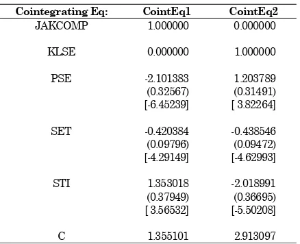
The results of the VECM estimation can be shown in the two consecutive tables. Table 2 (APPENDIX) shows the estimated cointegrating
vectors, whereas Table 3 report the coefficient of speed of adjustment.
Table 2. Estimated Cointegrating Vectors
Cointegrating Eq: CointEq1 CointEq2
JAKCOMP 1.000000 0.000000
KLSE 0.000000 1.000000
PSE -2.101383 1.203789
(0.32567) (0.31491)
[-6.45239] [ 3.82264]
SET -0.420384 -0.438546
(0.09796) (0.09472)
Note: cointegration with unrestricted intercepts and no trends. Included observations: 1948 after adjusting endpoints Standard errors in ( ) & t-statistics in [ ]
Table 3. Speed of Adjustment Parameter of the Error Correction Term (ECT)
Error Note : cointegration with unrestricted intercepts and no trends Included observations: 1948 after adjusting endpoints Standard errors in ( ) & t-statistics in [ ]
As a common practice, Table 2 (APPENDIX) shows that the first cointegrating vector is normalized by JAKCOMP, while KLSE is restricted to zero. Meanwhile, in the second one, KLSE is used to normalize, while JAKCOMP is restricted to zero. Based on t-statistic at the 5% level of significance, JAKCOMP, PSE, SET, and STI are found significant in the first cointegration vector, while KLSE, PSE, SET, and STI are significant in the second one. This means that all of the significant indices (variables) significantly contribute to the ASEAN indices’ long run equilibrium.
In contrast, the speed of adjustment of JAKCOMP, PSE, and STI are statistically significant in both vectors. JAKCOMP has negative influences in both cointegrating relationship indicating a downward long run adjustment. Conversely, STI affects the vectors positively implying an upward long run adjustment. In the second cointegrating vector, JAKCOMP will react to a disequilibrium among KLSE, PSE, SET, and STI. Thus, the vector would contribute to the convergence of JAKCOMP to its long run path, even though the index does not have any significant contribution to the others return to the long run equilibrium. PSE interestingly has positive and negative significant impact on the first and the second cointegration vectors, respectively. The implication is that PSE would react positively in the first vector, and negatively in the second one.
The existence of the cointegrating relationship in the region during the time period could be caused by some reasons. First, the degree of economic integration in the ASEAN countries has risen after the 1997 financial crisis. The information barriers have also significantly decline as a result of technological advance in IT (information technology) and in the markets’ trading operating systems. The other reason is that the degree of institutionalization and securitization have increased in the regional market promoting intra-regional fund transfers to increase diversification opportunities.
After the VECM estimation is determined, the next step is to search the existence of granger causality among variables of each model. The results of VEC Pairwise Granger Causality Tests for each country are presented Table 4. Using a 5% level of significance, the table shows only four significant causality linkages found among the variables in the pre crisis period. It also reveals that none of the other ASEAN indices is significantly granger caused JAKCOMP during the period, vice versa. Thus, it may be concluded that movements of the index during the period apparently become isolated from the influence of the others. STI experienced almost the same condition as JAKCOMP when all other ASEAN indices do not granger cause the index. However, somewhat different with JAKCOMP, STI, as well as SET, granger cause (in uni-directional form) KLSE meaning that movements in KLSE appeared to lag those of STI and SET. Moreover, SET also appears to have bi-directional causality with PSE.
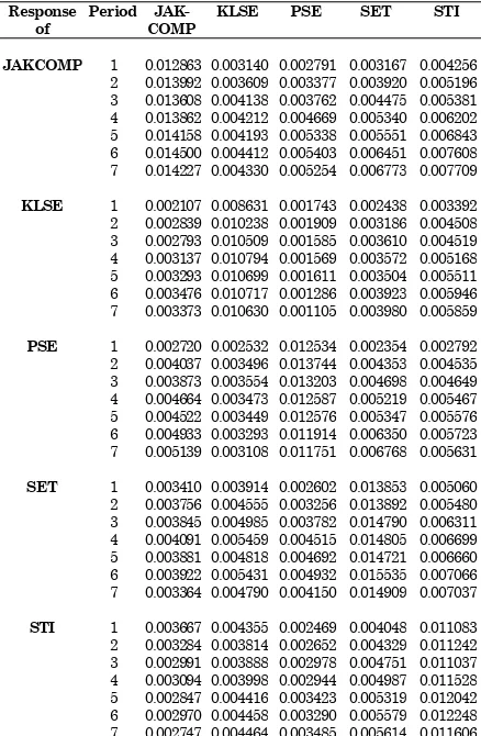
As a part of the Accounting Innovation Analysis, the impulse response analysis traces out the responsiveness of the dependent variable in the system to shocks to each of the variables (Brooks, 2002:341). The generalized type of the impulse response analysis will be applied in this study to
observe short run dynamic interactions among the variables, since orthogonalized impulse responses is sensitive to the ordering of the variable in the system. The complete result of the analysis is presented in Table 5.
Table 4. VEC Pairwise Granger Causality/Block Exogeneity Wald Tests
Dependent
variable Exclude Chi-sq Prob.
JAKCOMP KLSE 6.158533 0.4057
As can be seen in Table 5, a generalised impulse response analysis indicates that one standard error shock to JAKCOMP would result in a positive response by changes in STI of 0.0037, one step ahead. Afterward, the responses have become smaller ever since. A shock to STI, commonly believed as the most prominent stock index in ASEAN, results in second greatest changes in the other indices in the short run period. Meanwhile, the greatest contemporaneous reaction of an index generally due to its own shocks. This indicates that internal/domestic shocks in a particular index may have greatest significant impacts on its movements, and STI become the most influential stock index in the region at the time period.
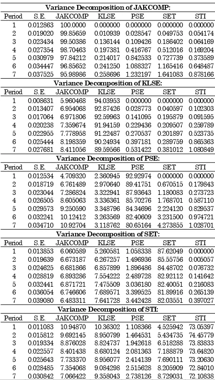
While impulse response functions trace the effects of a shock to one endogenous variable on to the other variables in the system, variance decomposition separates the variation in an endogenous variable into the component shocks to the system. As it is mentioned by Enders (2004:280) the forecast error variance decomposition tells the proportion of the movements in a sequence due to its own shock versus shock to the other variable.A shock to the
i-th variable will not only affect i-that variable, but can also be transmitted to all of the other variables in the system.
Table 6 presents the result of the forecast error variance decomposition of the serries in the period of before financial crisis. As can be seen from the table, in general, the proportion movements of the indices are dominantly due to their own shocks. Surprisingly, only around 70% of the error variance of STI was attributable to own shocks in the steps ahead, while JAKCOMP contributed maximum of 11% to STI’s error variance.
The Period of the 2007 Financial Crisis
The ADF test conducted to the serries at level reveals the presence of unit root in the serries. The lags order test then shows three lags length as the appropriate lag order since the residual is not serially correlated. However, the Johansen Cointegration test fails to find the existence of cointegration vector in the serries. This concludes that the serries has no cointegrating relationship. In other words, the indices have no long run equilibrium during the 2007 financial crisis. The finding somewhat contradicts with the ones given by some other researchers (Arshanapalli et al 1993; Sheng et al 2000, and Yang et al 2003), but confirms that of Roca (2000:145).
The absence of cointegrating vector in the series indicates that the cointegration analysis framework is not possible to be carried out. Hence, the VAR analysis framework would be applied to estimate the relationship of the indices, as well as to reveal the short run dynamic interactions among the indices.
Table 6. Variance Decomposition
Variance Decomposition of JAKCOMP:
Period S.E. JAKCOMP KLSE PSE SET STI
Variance Decomposition of KLSE:
Period S.E. JAKCOMP KLSE PSE SET STI
Variance Decomposition of PSE:
Period S.E. JAKCOMP KLSE PSE SET STI
Variance Decomposition of SET:
Period S.E. JAKCOMP KLSE PSE SET STI
Variance Decomposition of STI:
Period S.E. JAKCOMP KLSE PSE SET STI
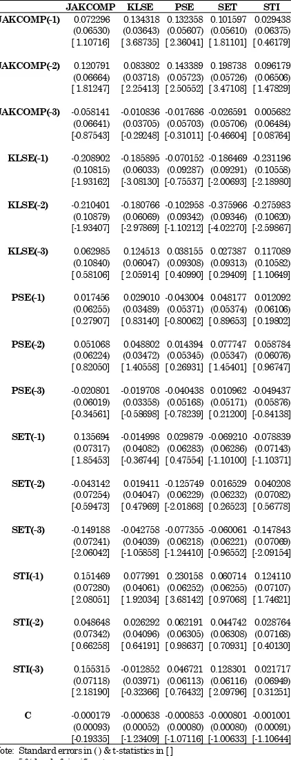
The VAR analysis, however, requires that the series must be stationary. Hence, the non stationary series may be made stationary by differencing or detrending process. After transforming the serries into first difference form, the ADF test is re-employed to ensure that the series are now stationary. The lag order test then indicated that the appropriate lag length would be three. After estimating the series using the VAR in first difference analysis, the estimated models can be shown in Table 7.
those indices in the region during the crisis period. The results are in fact different with those before the crisis period showing a changing behaviour in the indices’ movements. For instance, the lags of SET and STI now significantly enter into the equation for JAKCOMP, while in the pre crisis period does not.
Table 7. Vector Autoregression Estimates
JAKCOMP KLSE PSE SET STI JAKCOMP(-1) 0.072296 0.134318 0.132358 0.101597 0.029438
(0.06530) (0.03643) (0.05607) (0.05610) (0.06375) [ 1.10716] [ 3.68735] [ 2.36041] [ 1.81101] [ 0.46179]
JAKCOMP(-2) 0.120791 0.083802 0.143389 0.198738 0.096179 (0.06664) (0.03718) (0.05723) (0.05726) (0.06506) [ 1.81247] [ 2.25413] [ 2.50552] [ 3.47108] [ 1.47829]
JAKCOMP(-3) -0.058141 -0.010836 -0.017686 -0.026591 0.005682 (0.06641) (0.03705) (0.05703) (0.05706) (0.06484) [-0.87543] [-0.29248] [-0.31011] [-0.46604] [ 0.08764]
KLSE(-1) -0.208902 -0.185895 -0.070152 -0.186469 -0.231196 (0.10815) (0.06033) (0.09287) (0.09291) (0.10558) [-1.93162] [-3.08130] [-0.75537] [-2.00693] [-2.18980]
KLSE(-2) -0.210401 -0.180766 -0.102958 -0.375966 -0.275983 (0.10879) (0.06069) (0.09342) (0.09346) (0.10620) [-1.93407] [-2.97869] [-1.10212] [-4.02270] [-2.59867]
KLSE(-3) 0.062985 0.124513 0.038155 0.027387 0.117089 (0.10840) (0.06047) (0.09308) (0.09313) (0.10582) [ 0.58106] [ 2.05914] [ 0.40990] [ 0.29409] [ 1.10649]
PSE(-1) 0.017456 0.029010 -0.043004 0.048177 0.012092 (0.06255) (0.03489) (0.05371) (0.05374) (0.06106) [ 0.27907] [ 0.83140] [-0.80062] [ 0.89653] [ 0.19802]
PSE(-2) 0.051068 0.048802 0.014394 0.077747 0.058784 (0.06224) (0.03472) (0.05345) (0.05347) (0.06076) [ 0.82050] [ 1.40558] [ 0.26931] [ 1.45401] [ 0.96747]
PSE(-3) -0.020801 -0.019708 -0.040438 0.010962 -0.049437 (0.06019) (0.03358) (0.05168) (0.05171) (0.05876) [-0.34561] [-0.58698] [-0.78239] [ 0.21200] [-0.84138]
SET(-1) 0.135694 -0.014998 0.029879 -0.069210 -0.078839 (0.07317) (0.04082) (0.06283) (0.06286) (0.07143) [ 1.85453] [-0.36744] [ 0.47554] [-1.10100] [-1.10371]
SET(-2) -0.043142 0.019411 -0.125749 0.016529 0.040208 (0.07254) (0.04047) (0.06229) (0.06232) (0.07082) [-0.59473] [ 0.47969] [-2.01868] [ 0.26523] [ 0.56778]
SET(-3) -0.149188 -0.042758 -0.077355 -0.060061 -0.147843 (0.07241) (0.04039) (0.06218) (0.06221) (0.07069) [-2.06042] [-1.05858] [-1.24410] [-0.96552] [-2.09154]
STI(-1) 0.151469 0.077991 0.230158 0.060714 0.124110 (0.07280) (0.04061) (0.06252) (0.06255) (0.07107) [ 2.08051] [ 1.92034] [ 3.68142] [ 0.97068] [ 1.74621]
STI(-2) 0.048648 0.026292 0.062191 0.044742 0.028764 (0.07342) (0.04096) (0.06305) (0.06308) (0.07168) [ 0.66258] [ 0.64191] [ 0.98637] [ 0.70931] [ 0.40130]
STI(-3) 0.155315 -0.012852 0.046721 0.128301 0.021717 (0.07118) (0.03971) (0.06113) (0.06116) (0.06949) [ 2.18190] [-0.32366] [ 0.76432] [ 2.09796] [ 0.31251]
C -0.000179 -0.000638 -0.000853 -0.000801 -0.001001 (0.00093) (0.00052) (0.00080) (0.00080) (0.00091) [-0.19335] [-1.23409] [-1.07116] [-1.00633] [-1.10644] Note: Standard errors in ( ) & t-statistics in [ ]
5 % level of significant
Table 8. VAR Pairwise Granger Causality/Block Exogeneity Wald Tests
Dependent
variable Exclude Chi-sq Prob.
JAKCOMP KLSE 7.633367 0.0542 PSE 0.892896 0.8271 SET 7.966430 0.0467 STI 9.699188 0.0213
KLSE JAKCOMP 18.50092 0.0003 PSE 3.030814 0.3869 SET 1.542379 0.6725 STI 4.229433 0.2377
PSE JAKCOMP 11.80429 0.0081 KLSE 1.972551 0.5781 SET 5.832183 0.1201 STI 15.30169 0.0016
SET JAKCOMP 15.51245 0.0014 KLSE 19.47387 0.0002 PSE 2.766382 0.4291 STI 5.971454 0.1130
STI JAKCOMP 2.368227 0.4996 KLSE 12.88606 0.0049 PSE 1.790673 0.6170 SET 6.127043 0.1056
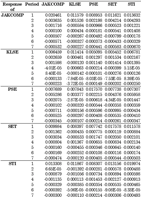
In order to capture the short run dynamic interaction among the variables during the financial crisis period, the generalized impulse response and the forecast error variance decomposition, would also be employed. The results of the generalized impulse response analysis of the series are presented in Table 9. As it is shown in the table, during the financial crisis, the generalised impulse response analysis indicates that all variables gave greater immediate reactions to a shock of one variable compared to those in the pre-crisis era. This implies that the short run interaction between two indices became more intense during the 2007 financial crisisperiod. In other words, the findings strongly indicate that the ASEAN indices become more interdependent during the financial crisis, although they had no long run equilibrium.
Table 9. The Impulse Response to Generalized 5 -0.000507 -0.000267 -0.000492 -0.000799 -0.000178 6 -0.000571 -0.000327 -0.000373 -0.000433 -0.000329 7 -0.000532 -0.000227 -0.000441 -0.000583 -0.000670
KLSE 1 0.006459 0.011414 0.005095 0.005452 0.006781 7 -0.000223 -3.72E-05 -0.000149 -0.000202 -0.000250
PSE 1 0.007689 0.007843 0.017570 0.007738 0.007307 2 0.005286 0.003377 0.002215 0.004376 0.005958 3 0.002075 -2.87E-05 0.000618 -4.34E-05 0.001447 4 -0.000102 -0.000320 -0.000544 -0.000358 0.000359 5 -0.000711 -0.000156 -0.000596 -0.000995 -0.000434 6 -0.000525 -0.000297 -0.000408 -0.000535 -0.000410 7 -0.000345 -0.000107 -0.000214 -0.000261 -0.000347
SET 1 0.009984 0.008397 0.007742 0.017578 0.011578 2 0.001362 -0.000435 0.000775 0.000119 0.000884 3 0.003034 -0.000533 0.001747 0.002050 0.002101 4 0.000804 0.001367 0.000655 0.000834 0.002134 5 -0.000160 -0.000455 -0.000346 -0.000645 -0.000140 6 -0.000169 -0.000252 -0.000108 -0.000116 0.000174 7 -0.000474 -0.000120 -0.000405 -0.000544 -0.000503
STI 1 0.013308 0.011867 0.008307 0.013156 0.019974 2 6.65E-05 -0.001392 -0.000281 -0.000578 0.000488 3 0.000879 -0.001056 0.000734 0.000894 0.000598 4 -0.001135 0.000113 -0.001453 -0.002127 -0.000913 5 -0.000329 -0.000385 -0.000354 -0.000535 -0.000465 6 -0.000392 -5.06E-05 -0.000155 -9.08E-05 -8.33E-05 7 -0.000300 -0.000110 -0.000214 -0.000306 -0.000493
Table 10. Variance Decomposition
Variance Decomposition of JAKCOMP:
Period S.E. JAKCOMP KLSE PSE SET STI
Variance Decomposition of KLSE:
Period S.E. JAKCOMP KLSE PSE SET STI
Variance Decomposition of PSE:
Period S.E. JAKCOMP KLSE PSE SET STI
Variance Decomposition of SET:
Period S.E. JAKCOMP KLSE PSE SET STI
Variance Decomposition of DLNSTI:
Period S.E. JAKCOMP KLSE PSE SET STI
The study concludes that two cointegrating vectors are found in the series before the 2007 financial crisis period indicating the existing of long run equilibrium in the series during the time period. However, the study fails to find any cointegrating vector in the series during the financial crisis period. The results prove that the long run relationship of the ASEAN indices has been removed by the 2007 financial crisis.
The block causality tests employed in both sub-sample period reveal that more significant causal linkages are found in the series during the financial crisis period compared to those before the financial crisis. The accounting innovation analyses conducted to the series also indicate that the short run dynamic interactions among the indices tend to be more intense during the financial crisis period. These all indicate that the indices become more interdependent during the financial crisis period since the moment gives rise the explanatory power of a sequence to the movements of another.
The general conclusion that may be withdrawn from this study is that the contagious effect of the 2007-US financial crisis has affected the ASEAN’s capital market integration, and has changed the behaviour of the indices’ movements both in the short run and in the long run.
Thus, the implication policy that can be suggested is that the diversification of portfolio within the ASEAN stock markets in the short run is unlikely to reduce the risk due to the high degree of financial interdependent of these markets during the financial crisis.
REFERENCES
Arshanapalli, B. and Doukas, J. 1993, ‘International Stock Market Linkages: Evidence from the pre- and post-October 1987 Period’, Journal of Banking and Finance, 17 (1): 193-208.
Arshanapalli, B., Doukas, J. and Lang, L. 1995, ‘Pre and post-October1987 Stock Market Linkages between U.S and Asian markets’,
Brailford, T., Heaney, R. and Bilson, C. 2004.
Investment: Concepts and Applications,
Second Edition. Thomson Learning:
Australia.
Brooks, C. 2002. Introductory Econometrics for Finance. Cambrige University Press: Cambrige.
Chan, K.C., Gup, B.E. and Pan, M. 1992, ‘An Empirical Analysis of Stock Prices in Major Asian Markets and the United States’,
Financial Review, 27 (2): 289-307.
Chung, P. and Liu, D. (1994), ‘Common Stochastic Trend in Pacific Rim Stock Markets’,
Quarterly Review of Economics and Finance, 34: 241-259.
Climent, F. and Meneu, V. 2003, ‘Has 1997 Asian Crisis Increased Information Flows between International Markets’, International Review of Economics and Finance, 12(1): 111-143.
DeFusco, R.A., Geppert, J.M. and Tsetsekos, G.P. (1996), ‘Long-run Diversification Potential in Emerging Stock Markets’, Financial Review, 31(2): 343-363.
Dekker, A., Sen, K. and Young, M. 2001. ‘Equity Market Linkage in the Asia Pacific Region: A Comparison of the Orthogonalized and Generalized VAR Approaches’. Global Finance Journal, 12: 1-33.
Department of Foreign Affair and Trade of Australia (DFAT). 1999, Asia’s Financial Markets: Capitalising on Reform, East Asia Analytical Unit, Canberra.
Enders, W. (2004). Applied Econometric Time Series: Second Edition. John Wiley & Sons: USA.
Eun, C.S. and Shim, S. 1989, ‘International Transmission of Stock Market Movements’,
Journal of Financial and Quantitative Analysis, 24 (2): 241-56.
Hung, B. and Cheung, Y. 1995, ‘Interdependence of Asian Emerging Equity Markets’, Journal of Business Finance and Accounting, 22 (2): 281-88.
International Monetary Fund 2004. International Financial Statistic (IFS) Online. Washington DC.
Johansen, S. and Juselius, K.. 1990, ‘The Full Information Maximum Likelihood Procedures for Inference on Cointegration with Applications to the Demand for Money’,
Oxford Bulletin of Economics and Statistics, 52(2): 169-210.
Kasa, K. 1992, ‘Common Stochastic Trends in International Stock Markets’, Journal of Monetary Economics, 29: 95-124.
Kenen, P.B. 1976, ‘Capital Mobility and Integration: A Survey’, Princeton Studies in International Finance No. 39, Princeton University: USA.
King, M and Wadwhani, S. 1990, ‘Transmission of Volatility between Stock Markets’, Review of Financial Studies, 3 (1): 5-33.
Krugman, P.R. and Obstfeld, M. 2003. Inter-national Economics: Theory & Policy 6th
Edition. The Addison-Wesley: Boston.
Liu, Y.A., Pan, M.S. and Shieh, J.C.P. 1998, ‘International Transmission of Stock Price Movements: Evidence from the U.S. and Five Asian-Pacific Markets’, Journal of Economics and Finance, 22 (1): 59-69.
Lutkepohl, H. and Reimers, H.E. 1992. ‘Impulse Response Analysis of Cointegrated System’,
Journal of Economic Dynamics and Control, 16: 53-78.
Masih, A.M.M. and Masih, R. 1999, ‘Are Asian Stock Markets Fluctuations Due to Mainly to Intra-regional Contagion Effects? Evidence Based on Asian Emerging Markets’, Pacific-Basin Finance Journal, 7 (3): 251-82.
Masih, R. and Masih, A.M.M. 2001, ‘Long and Short-term Dynamic Causal Transmission amongst International Stock Markets’,
Journal of International Money and Finance, 20: 563-87.
Palac-McMiken, E.D. 1997, ‘An Examination of ASEAN Stock Markets: a Cointegration Approach’. ASEAN Economic Bulletin, 13 (3): 299-311.
Pretorius, E. 2002, ‘Economic Determinants of Emerging Market Stock Market Inter-dependence’, Emerging Markets Review, 3: 84-105.
Roca, E.D. 2000, Price Interdependence among Equity Markets in the Asia-Pacific Region: Focus on Australia and ASEAN, Ashgate: Aldershot.
Sachs, J.D and Larrain, F. B. 1993, Macro-economics in the Global Economy, Prentice Hall: New Jersey.
Serletis, A. and King, M. 1997, ‘Common Stochastic Trends and Convergence of European Union Stock Markets’, The Manchester School, 65(1): 44-57.
Sheng, H. and Tu, A. 2000, ‘A Study of Cointegration and Variance Decomposition among National Equity Indices before and during the Period of the Asian Financial Crisis’, Journal of Multinational Financial Management, 10 (3): 345-65.
Stulz, R. 1981, ‘On the Effects of Barriers to International Investment’, Journal of Finance, 36: 923-934.
Thomas, R.L 1997. Modern Econometrics: an Introduction. Addison-Wesley: Harlow.
Yang, J., Kolari, J.W. and Min, I. 2003, ‘Stock Market Integration and Financial Crises: the Case of Asia’, Applied Financial Economics, 13: 477-486.