Development of Total Suspended Sediment Model using Landsat-8 OLI and
In-situ Data at the Surabaya Coast, East Java, Indonesia
Teguh Hariyanto, Trismono C. Krisna, Khomsin, Cherie Bhekti Pribadi and Nadjadji
Anwar
Received: 09 02 2016 / Accepted: 27 06 2016 / Published online: 30 06 2017 © 2017 Faculty of Geography UGM and he Indonesian Geographers Association
Abstract he decrease of coastal-water quality in the Surabaya coastal region can be recognized from the conceentra-tion of Total Suspended Sediment(TSS ) . As a result we need a system for monitoring sediment concentraconceentra-tion in the coastal region of Surabaya which regularly measures TSS. he principle to model and monitor TSSconcentration using remote sensing methods is by the integration of Landsat-8OLI satellites image processing using some ofTSS-models then those are analyzed for looking its suitability with TSS value direcly measured in the ield ( in-situ measurement). he TSS value modeled from all algorithms validated usingcorrelation analysis and linear regression . he result shows that TSS model with the highest correlation value is TSS algorithm by Budiman (2004)with r value 0.991. Hence this algorithm can be used to investigate TSS-distribution which represent the coastal water quality of Surabaya with TSS value between 75 mg/L to 125 mg/L.
Abstrak Penurunan kualitas perairan pantai dapat ditunjukkan oleh tingginya konsentrasi sedimen yang dinyatakan oleh
Total Suspended Sedimen(TSS). Untuk keperluan ini diperlukan sistem monitoring dan pengukuran konsentrasi sedimen wilayah pantai Surabaya secara spasial dan non spasial, dimana pengukuran TSS dapat dilakukan secara regular dengan ketelitian yang baik. Prinsip monitoring konsentrasi TSS dengan metode penginderaan jauh adalah memproses citra dari satelit Landsat 8OLI dengan menggunakan beberapa model TSS, kemudian dilihat kesesuaiannya konsentrasi TSS yang diukur langsung di lapangan (pengukuran insitu).Penelitian ini menggunakan empat algoritma TSS untuk mendapatkan konsentrasi TSS. Nilai konsentrasi TSS dari semua algortima diuji dengan data in-situ menggunakan analisis regresi linier. Hasil menunjukkan bahwa algoritma Budiman mempunyai nilai korelasi yang paling tinggi(r=0,991).Algoritma tersebut dapat digunakan untuk melihat distribusi TSS yang merupakan indikator kualitas perairan pantai Surabaya dengan rent-ang nilai konsentrasi 75 mg/l sampai dengan 125 mg/l.
Keywords: algorithm, coastal water, Landsat 8 OLI, Total Suspended Sediment (TSS), Surabaya
Kata kunci: algoritma, Landsat 8 OLI, Total Suspended Sediment (TSS), perairan pantai, Surabaya
1.Introduction
Coastal areas oten change in their function , the area which should be the conservation area or coastal protection, forests , as well as water catchment areas and mangrove forest habitat have been transformed into large scale residential area, industrial area, warehousing and others that have negative impacts on that region. Several cases of coastal reclamation area can be seen in coastal areas of Jakarta, as in the spatial plan of the city, the northern coastal region of Jakarta is designated as protected forest or mangrove forests, but in fact that region has been developed to be come residential area. As a result this triggers looding in the wider regions. Form example,reclamation is a necessity for the development of the capital Jakarta, that aims to expand the area used for economic activities. Likewise in the case of the Surabaya east coast region, the reclamation was inluenced by several factors
Teguh Hariyanto, Trismono C. Krisna, Khomsin, Cherie Bhekti Pribadi and Nadjaji Anwar
Faculty of Civil Engineering and Planning, Institut Teknologi Sepu-luh Nopember Surabaya.
Correspondent email: [email protected].
for instance the demand of residential areas , factories and so on, as well as due to the sedimentation in the river estuary which resulted in the emergence of ‘new land’. he impact of the reclamation both technically (backilling) or natural (newland) certainly have impacts either positively or negatively [Hariyanto,2014].
Monitoring the condition of the coast through TSS value change using Landsat-8 OLI (Operational Land Imager) satellite remote sensing in the Surabayaeast coast area is necessary since there are some important things to be noted as a result of the reclamation either technically or naturally (new land). he efects of the reclamation are coastline changes, social issues, population and others. Furthermore we need the update of TSS data which is necessary to determine operational policy and technical guidance for the government, public and private sector in the utilization of coastal region from occurring environmental changes
he utilization of TSS remote sensing models in the previous study was performed by Budiman [2004], Nurandani [2013] , Lestari [2009], and Rodriguez and Gilbes [2009]. Initial hypothesis is applied to obtain the highest correlation and best-it linear regression equation
Indonesian Journal of Geography Vol. 49, No.1, June 2017 (73- 79)
of the TSS distribution to represent the condition of Surabaya coastal-water with 15 in-situ data sample.he TSS model which has correlation value close to 1 will be used as the basis for analyzing coastal water condition
he aims of this research are retrieveand evaluate TSS concentration distribution using four algorithms of TSS in Surabaya east coast from Landsat-8 OLI image. Evaluate TSS correlation result retrieved from four algorithms against in-situ data using correlation value (r) and linier regression analysis.he best result will be used as the basis to explains the condition of Surabaya east coast
2.he Methods
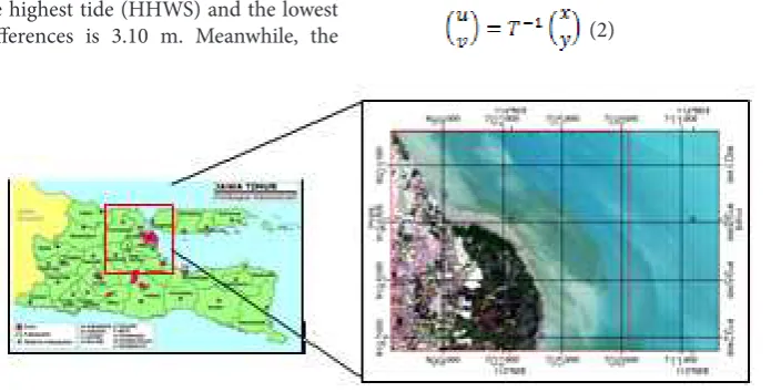
Research location is in the East Coast of Surabayawhich has a center coordinate of 7o15’20”
South and 112049’50” East (Figure 1). he Sea region
of Surabaya is divided into two zones, the irst zone is the strait and located in the northern part while the second zone is the sea zones located in the eastern part. Both zones have diferent sea level characteristics caused by the ocean currents. Madura Strait is a narrow strait which connects the Java and Madura island. Java sea (southern part of Madura) in average has strong current which is 0.5 m and 0.6 m/s at the surface and at the bottom of strait respectively. Tidal conditions on the north coast of Surabaya is Semi-Diurnal with the highest tide (HHWS) and the lowest tide (LLWS) diferences is 3.10 m. Meanwhile, the
sea level condition on the east coast of Surabaya has the characteristics of Semi Diurnal (two tide per day) with the highest tide (HHWS) and the lowest tide (LLWS)diferences of 2.80 m with strong currents 0.4 m/s on the surface and 0.48 m/s at the bottom of the sea. Due to the sea level conditions in the eastern part of Surabaya, the occurrence of sedimentation is more likely compared to the northern part.
he spectral characteristics of Landsat 8 OLI is provided in Table 1. Landsat-8 OLI image used in this study was acquired on March 3, 2014 with the number of pat-119 and row- 065, the spatial resolution is 30mx30m. Image-to-image registration is the matching of one image to another so the same geographic area is positioned coincident with respect to the other. his type of geometric correction is used when it is not necessary to have each pixel assigned a unique x, y coordinate in a map projection [Baboo, 2011] (Figure 2) In order toget :
(1)
Every step involved in the imaging process has to be known, i.e., we need to know the inverse process of geometric transformation.
(2)
Figure 1. Research location, Surabaya east coast. (Source: East Jawa Administration Map and Landsat 8 OLI)
Figure 2. Image to image registration geometric correction.
his is a complex and time consuming process. However, there is a simpler and widely-used alternative, the polynomial approximation.
(3)
(4)
Coeicients a’s and b’s are determined by using Ground Control Points (GCPs). For example, we can use very low order polynomials such as the aine transformation.
(5)
(6)
A minimum of three GCPs will enable us to determine the coeicients in the above equations.herefore, we did not need to use the transformation matrix T. However, in order to make our coeicients representative of the whole transformed image, we have to make sure that our GCPs are well distributed across the image [Camper, 2011]he distance between the input location of the GCP and the retransformed coordinates of the same GCP is called the Root Mean Square (RMS) error. his is calculated in the rectiication formula as follows (see Table 2 for the result)
(7)
(8)
(9)
Where :
Rx = X RMS Error Ry = Y RMS Error T = Total RMS Error n = the number of GCPs
i = GCP number
XRi = the X residual for GCPi YRi = the Y residual for GCPi
TSS in-situ Data.
In-situ data came from water samples on the East Coast of Surabaya when were taken at March 24, 2014 by the random sampling method as much as 15 points in the study site at a depth of 0.5 - 2 m .Furthermore water samples were processed using Gravimetry method in Water Laboratory of Environmental Engineering - ITS to obtain the value of TSS .
Radiometric Correction
Landsat 8 OLI band data can also be converted to Top-of-Atmospheric(TOA) planetary relectance using relectance rescaling coeicients provided in the product metadata ile (MTL ile). he following equation is used to convert DN values to TOA relectance for Landsat 8 OLI data:
(10)
where:
ρλ’ = TOA planetary relectance, with no correction Table 1. Landsat-8 (OLI) spectral band [Edgardh, 2013]
Band Wavelength (µm) Resolution (m)
B1-Visible (Aerosol) 0.43 - 0.45 30
B2-Visible 0.45 - 0.51 30
B3-Visible 0.45 - 0.51 30
B4-NIR 0.53 - 0.59 30
B5-NIR 0.64 - 0.67 30
B6-SWIR1 0.85 - 0.88 30
B7-SWIR2 1.57 - 1.65 30
B8-PAN 2.11 - 2.29 15
B9-Cirrus 0.50 - 0.68 30
B10-TIRS1 1.36 - 1.38 100
B11-TIRS2 10.60 100
for solar angle
Mρ= Band-speciic multiplicative rescaling factor taken from the image metadata (REFLECTANCE_ MULT_BAND_x, where x is the band number) Aρ= Band-speciic additive rescaling factor taken from the image metadata (REFLECTANCE_ADD_ BAND_x, where x is the band number)
Qcal= DN
To obtainTOA relectance value with a correction for the sun angle, the following formula was used
(11)
where:
ρλ = TOA planetary relectance
θSE = Local sun elevation angle. he value of scene center sun elevation angle in degrees is provided in the metadata (SUN_ELEVATION)
θSZ = Local solar zenith angle; θSZ = 90° - θSE
Some models of TSS algorithm used in this study can be seen in the following explanation
3. Result and discussion.
Budhiman [2004] method is based on bio optical modeling. he forward water analysis comprised the laboratory measurements of water quality (TSS and Chlorophyll) and Inherent Optical Properties (IOPs) to derive Speciic Inherent Optical properties (SIOPs). SIOPs of water (TSM, Chlorophyll and CDOM), coeicient f and B were used to developed R(0-) model. he inverse atmosphere analysis encompassed several image pre-processing procedures (i.e geometric correction, atmospheric correction, air-water interface correction). he last step is the inverse water analysis, which comprised the development of algorithm and image processing to develop TSS concentration maps. he results indicate that red band of satellite sensor is sensitive to detect higher TSS concentration. Green band is sensitive to detect the lower TSS Table 2. he result of geometric correction (pixel).
GCP Base X Base Y Warp X Warp Y Predict X Predict Y Error X Error Y RMS
1 3041.75 2366.25 2766.00 4845.50 2765.867 4845.580 -0.1334 0.0796 0.155
2 2662.50 2554.25 2385.75 5035.50 2385.758 5035.491 0.0082 -0.0091 0.012
3 2713.00 2330.00 2436.50 4810.25 2436.449 4810.284 -0.0509 0.0337 0.061
4 2664.24 2779.00 2367.50 5261.00 2367.440 5261.039 -0.0603 0.0387 0.072
5 3140.50 2813.50 2863.50 5295.25 2863.424 5295.296 -0.0758 0.0457 0.089
6 2943.50 2543.75 2666.75 5024.50 2667.060 5024.312 0.3096 -0.1885 0.362
7 3160.75 2536.75 2884.56 5016.77 2884.563 5016.770 0.0026 -0.0001 0.003
RMS Error Total 0.157
Table 3. TSS insitu laboratory data measured using Gravimetry method No. Point TSS (mg/L) X (m) Y (m)
1 44 704337 9193046
2 29 702649 9200424
3 62 704384 9195010
4 29 704114 9199646
5 94 703323 9196945
6 36 703355 9198889
7 30 705283 9198413
8 34 699994 9200567
9 47 701568 9199269
10 40 701357 9201597
11 24 706292 9192318
12 28 706088 9194229
13 35 699700 9202008
14 76 706385 9195644
concentration. For Mahakam Delta, red band algorithm was used to derive TSS map, since higher TSS concentration occurred in the delta.he result can be seen in Figure 3 and the formula is as follow,
(12)
where :
x= relextance of Band 3 (red)
TSS Algorithm 2 : Nurandani [2013]
Based on Nurandani [2013], who observed and measured TSS in Rawa Pening, the results of data processing , empirical matching algorithm for the concentration of TSS is a logarithmic regression equation model using the ratio between band 1 (blue) with band 2 (green) of Landsat 7 ETM+.herefore it changes into band 2 (blue) and band 3 (green) on Landsat-8 OLI respectively. he equation is as follow:
(13)
where :
x = Relectance Ratio betwen band 2 and band 3 he majority of TSS value is between 75-100 mg/L, which covers almost all of the study area, while the value of TSS between 50-75 mg/L is distributed in Madura Strait.Using this algorithm , there is only limited area with TSS value between 25-50 mg/L.he TSS map can be seen in Figure 4.
TSS algorithm 3: Lestari [2009]
Based on Lestari [2009], the best empirical model to predict the concentration of TSS is the 3rd degree polynomial regression model, both for the dry and rainy seasons. he model is created by the relationship between the chromaticity transformation relectance values of blue band with TSS concentration in-situ data. Here is the formula:
TSS(mg/l)=24197x3-22050x2+6813x-644.98 (14)
Figure 3. TSS map distribution using Budhiman [2004] algorithm.
Figure 4. TSS map distribution using Nurandhani [2013] algorithm.
Figure 5. TSS distribution map using Lestari [2009] algorithm
Table 4. TSS and insitu data value
X Y Insitu TSS 1 TSS 2 TSS 3 TSS 4
704337 9193046 44 134.5768 68.26647 37.70394 76.03919
702649 9200424 29 123.707 56.95261 36.65344 63.01086
704384 9195010 62 151.1878 69.24554 40.01199 77.60974
704114 9199646 29 120.8465 56.90761 36.51542 62.26074
703323 9196945 94 174.1747 72.03088 40.62543 79.58472
703355 9198889 36 125.9703 65.10379 37.51991 73.6571
705283 9198413 30 124.2871 61.22649 36.90648 66.31433
699994 9200567 34 124.724 61.58656 37.31288 71.10242
701568 9199269 47 139.628 68.74805 38.11801 76.21643
701357 9201597 40 130.6984 67.49869 37.55825 74.63062
706292 9192318 24 115.1877 55.3726 35.8253 60.07251
706088 9194229 28 115.39 55.79576 35.83297 61.91773
699700 9202008 35 125.6025 64.78537 37.45857 71.74793
706385 9195644 76 161.5173 70.73078 40.28037 79.48254
706024 9197009 60 143.8556 69.20729 38.83112 76.26843
Figure 7. Linear regression analysis between TSS insitu over TSS retrieved using Budhiman [2004]
algorithm.
Figure 8. Linear regression between TSS insitu over TSS modeled using nurandani [2013] algorithm.
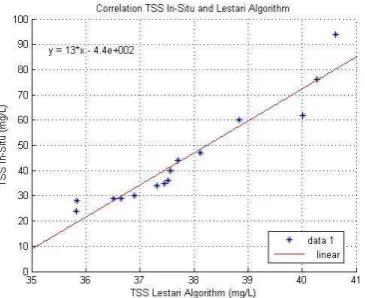
Figure 9. Linear regression between TSS insitu over TSS retrieved using Lestari [2009] algorithm.
Figure 10. Linear regression between TSS insitu over TSS retrieved using Rodriguey and Gilbes [2009]
where :
x= relectance of blue band l chromaticity. according to Wouthuyzen et al. (2008) in Lestari (2009), blue band chromaticity is : (band 2 / (band 2+band 3+band 4)
TSS distribution obtained usingLestarialgorithm can be seen in ig.10 where the TSS value appears in the range of 25-50 mg/L TSS algorithm 4 : Rodriguez and Gilbes (2009). he result of Rodriguez and Gilbes (2009) algorithm shown in Figure 6 produced 3 broadest TSS value ranges.TSS range of 75-100 mg/L which covers the largest area, while the next largest TSS value is between 50-75 mg/L and the smallest area of TSS value is between 100-125 mg/L .he formula is as follow :
TSS=602.63*(05157*x-0.0089+3.1481 (15)
where :
x = relectance band 2
Figure 7 explain the regression analysis between the TSS in-situ data over the TSS retrieved using Budhiman [2004] algorithm, where it has a good density at the sample number 3, 6 and 7 as well as at 8 and 9. herefore, it has a high value of R2 = 0.982, while the correlation value (r) is 0.991. Figure 8 explains regression analysis between the TSS insitu data over TSS retrieved using Nurandani [2013] algorithm, where the highest density is at the sample number 11. From the calculation it has R2 of 0.684 and r of 0.827. Figure 9 explains the regression analysis between TSS insitu data with TSS modeled using Lestari [2009] algorithm, where good density appeared at sample number 3, 4, 10 , 11 and 13.he value of R2 is 0.915 while the value of r is 0.957. Figure 10 explains the regression analysis between the TSS in-situ data with TSS modeled using Rodriguez and Gilbes [2009] algorithm, where the relationship is quite poor R2 of 0.652 and r of 0.807. Based on analysis test for all TSS models using linear regression method, the maximum r value was obtained from Budiman algorithm with r = 0.991. Hence the water condition in the eastern coast of Surabaya based on the results of Budiman’s [2004] TSS algorithm has the biggest range of TSS value between 100-125 mg/L.he value of 125 mg/L are located in the edge of the coastline indicating the new land formation as a result of the sedimentation process .
4.Conclusion
he use of fourt TSS algorithms applied to Landsat-8 OLI result in the TSS distribution vary from 40 mg/L up to 150 mg/L, where the highest variety of TSS value was obtained using Budiman [2004] algorithm, whereas the lowest TSS value is obtained using Lestari [2009)] Nurandani [2013] and Rodriguez and Gilbes [2009] algorithms produced almost similar TSS valuesUsing four TSS algorithms above, model with the highest correlation with TSS Budhiman [2004] algorithm
with r value 0f 0.991. he lowest correlation value was obtained from Rodriguez and Gilbes [2009] algorithm. he concentration of TSS in the east coast of Surabaya based on Budiman algorithm which has the largest value of 125 mg/L, are distributed on the edge of the coastline, and thus increasing sedimentation process.
References
Baboo.S.S, (2011). Geometric Correction in Recent High Resolution Satellite Imagery : A Case Study in Coimbatore, International Journal of Computer Applications ,Volume 14– No.1, 0975 – 8887. Budhiman, S, (2004). Mapping TSM Concentrations From
Multi Sensor Satellite Images in Turbid Tropical Coastal Waters of Mahakam Delta Indonesia, Enschede: MSc hesis ITC Enschede, he Netherlands. Camper, (2011). Georeferencing (Geometric
Correction), Remote Sensing and Image Analysis, University of California at Berkeley. Edgardh.L.A, Landsat 8, LDCM Landsat
data Continuity Mission NASA – USGS. Hariyanto,T, (2014). Identiication of Total Suspended Sediment (TSS) Distribution at Surabaya East Coast Area in East Java Indonesia Using TSS Algorithm Implementation on Multi Temporal Satellite Images, International Journal of Earth Sciences and Engineering ISSN 0974-5904, Vol. 07, No. 04, August, 2014, pp. 1341-1346 Nurandani.P. (2013). Pemetaan Total Suspended Solid (TSS)
Menggunakan Citra Satelit Multi Temporal di Danau Rawa Pening Provinsi Jawa Tengah. Teknik Geodesi Undip. Rodriguez-Guzman,V. And Gilbes .F.(2009). Using Modis
![Table 1. Landsat-8 (OLI) spectral band [Edgardh, 2013]](https://thumb-ap.123doks.com/thumbv2/123dok/3668144.1803494/3.595.72.531.67.311/table-landsat-oli-spectral-band-edgardh.webp)
![Figure 5. TSS distribution map using Lestari [2009]](https://thumb-ap.123doks.com/thumbv2/123dok/3668144.1803494/5.595.75.524.561.728/figure-tss-distribution-map-using-lestari.webp)