Bidif ferential Calculus Approach
to AKNS Hierarchies and Their Solutions
Aristophanes DIMAKIS † and Folkert M ¨ULLER-HOISSEN ‡
† Department of Financial and Management Engineering, University of the Aegean,
41, Kountourioti Str., GR-82100 Chios, Greece
E-mail: [email protected]
‡ Max-Planck-Institute for Dynamics and Self-Organization,
Bunsenstrasse 10, D-37073 G¨ottingen, Germany
E-mail: [email protected]
Received April 12, 2010, in final form June 21, 2010; Published online July 16, 2010 doi:10.3842/SIGMA.2010.055
Abstract. We express AKNS hierarchies, admitting reductions to matrix NLS and matrix mKdV hierarchies, in terms of a bidifferential graded algebra. Application of a universal result in this framework quickly generates an infinite family of exact solutions, including e.g. the matrix solitons in the focusing NLS case. Exploiting a general Miura transformation, we recover the generalized Heisenberg magnet hierarchy and establish a corresponding solution formula for it. Simply by exchanging the roles of the two derivations of the bidifferential graded algebra, we recover “negative flows”, leading to an extension of the respective hierar-chy. In this way we also meet a matrix and vector version of the short pulse equation and also the sine-Gordon equation. For these equations corresponding solution formulas are also derived. In all these cases the solutions are parametrized in terms of matrix data that have to satisfy a certain Sylvester equation.
Key words: AKNS hierarchy; negative flows; Miura transformation; bidifferential graded algebra; Heisenberg magnet; mKdV; NLS; sine-Gordon; vector short pulse equation; matrix solitons
2010 Mathematics Subject Classification: 37J35; 37K10; 16E45
1
Introduction
A unification of some integrability aspects and solution generating techniques has recently been achieved for a wide class of “integrable” partial differential or difference equations (PDEs) in the framework of bidifferential graded algebras [1]. The hurdle to take is to find a bidifferential calculus (i.e. bidifferential graded algebra) associated with the respective PDE. In particular, a surprisingly simple result (Theorem 3.1 in [1] and Theorem1below) then generates a (typically large) class of exact solutions. This has been elaborated in detail for matrix NLS systems in a recent work [2]. The present work extends some of these results to a corresponding hierarchy and moreover to related hierarchies. It demonstrates how to deal with whole hierarchies instead of only single equations or systems in the bidifferential calculus approach and shows moreover that certain relations between hierarchies find a nice explanation in this framework. Except for certain specializations, we deal with “non-commutative equations”, i.e. we treat the dependent variables as non-commutative matrices, and the solution formulas that we present respect this fact.
bidifferential calculus framework, a “reciprocal” [3] or “negative” extension of the hierarchy naturally appears. “Negative flows” have been considered previously via negative powers of a recursion operator (see e.g. [4, 5, 6, 7] and also [8, 9, 10, 11] for other aspects). In our picture, these rather emerge as “mixed equations”, bridging between the ordinary hierarchy and a “purely negative” counterpart.
Section6elaborates this program for a “dual hierarchy”. Here we recover in the bidifferential calculus framework in particular a well-known duality or gauge equivalence between the (matrix) NLS and (generalized) Heisenberg magnet hierarchies [12,13, 14,15,16,17,18,19]. Section7
contains some concluding remarks.
2
Basic structures
Definition 1. Agraded algebra is an associative algebra Ω overCwith a direct sum decompo-sition
Ω =M
r≥0
Ωr
into a subalgebra A= Ω0 and A-bimodules Ωr, such that
ΩrΩs⊆Ωr+s.
Definition 2. A bidifferential calculus (or bidifferential graded algebra) is a graded algebra Ω equipped with two (C-linear) graded derivations d,¯d : Ω→Ω of degree one (hence dΩr ⊆Ωr+1, ¯
dΩr ⊆Ωr+1), with the properties
d◦d = 0, ¯d◦d = 0¯ , d◦¯d + ¯d◦d = 0,
and the graded Leibniz rule
d(χχ′) = (dχ)χ′+ (−1)rχdχ′, d(¯ χχ′) = (¯dχ)χ′+ (−1)rχ¯dχ′,
for all χ∈Ωr and χ′ ∈Ω.
For any algebraA, a corresponding graded algebra is given by
Ω =A ⊗^ CN, (2.1)
whereV(CN) denotes the exterior algebra ofCN,N >1. Defining graded derivations d, ¯d onA, they extend in an obvious way to Ω such that the Leibniz rule holds and elements of V(CN) are treated as constants with respect to d and ¯d.
Given a bidifferential calculus, it turns out that the equation
¯
ddφ= dφ∧dφ, where φ∈ A, (2.2)
has various integrability properties [1, 2]. By choosing a suitable bidifferential calculus, this equation covers in particular the familiar selfdual Yang–Mills equation (in one of its gauge-reduced potential versions), but also e.g. discrete integrable equations [1,2]. In the next section we demonstrate that, by choosing an appropriate bidifferential calculus, (2.2) reproduces matrix AKNS hierarchies.
The (modified)Miura transformation
where ¯d∆ = (d∆)∆, is a hetero-B¨acklund transformation between (2.2) and thedual equation1
d [¯dg−(dg)∆]g−1= 0. (2.4)
In the present work we concentrate on the case where ∆ = 0. We note that (2.3) and (2.4) are equivalent if d has trivial cohomology. But this is in general not the case.
Exchanging d and ¯d in (2.2), we get a different equation. Dealing with hierarchies, such an exchange leads to what we call the reciprocal hierarchy. If ∆ = 0, exchanging d and ¯d in (2.4), simply amounts to replacing g byg−1.
3
AKNS hierarchies
Let B0 be the algebra of complex smooth functions of independent variables t1, t2, t3, . . .,B an
extension by certain operators (specified below), and A = Mat(m, m,B), m > 1. Let m = m1+m2 withmi ∈N, and let P be the projection
P =P(m1,m2) =
Im1 0m1×m2 0m2×m1 0m2×m2
, (3.1)
where Im denotes the m×m identity matrix. If the dimension is obvious from the context, we
will simply denote it byI. It will also be convenient to introduce the matrix
J =J(m1,m2)= 2P −Im.
3.1 NLS system
A particular bidifferential calculus onA is determined by
df = [P, f]ζ1+ [P∂x, f]ζ2, ¯df =fxζ1+1
2[∂t2 +∂
2
x, f]ζ2, (3.2)
whereζ1,ζ2 is a basis ofV1(C2), and we setx=t1. HereBis the extension ofB0 by the partial
derivative operator∂x. Evaluation of (2.2) yields
[P, φt2] ={P, φxx}+ 2(Pφx)[P, φ]−2[P, φ]φxP, (3.3)
using the familiar notation for commutator and anti-commutator. The block-decomposition
φ=J
p q ¯ q p¯
=
p q
−q¯ −p¯
, (3.4)
(where p, ¯p,q, ¯q have size m1×m1,m2×m2,m1×m2,m2×m1, respectively), results in the
NLS system2
qt2 =qxx−2qqq,¯ q¯t2 =−q¯xx+ 2¯qqq,¯ (3.5)
together with
px =−qq,¯ (3.6)
where we set a “constant” of integration to zero. As a consequence of the form of P, there is no equation for ¯p. Though at this point we could simply set it to zero, this would be inconsistent with further methods used in this work (cf. Remark3).
1
IntroducingB= [¯dg−(dg)∆]g−1
, this equation reads dB= 0, and as a consequence, taking also ¯d∆ = (d∆)∆ into account, we find that ¯dB =B∧B. If, as in familiar cases, this (partial) zero curvature equation implies B = (¯dg′)g′−1
, then (2.4) is gauge-equivalent to d[(¯dg′)g′−1
] = 0, so that the term involving ∆ in (2.4) can be generated by a gauge transformation. It is nevertheless helpful to consider the modified equation (2.4) in order to accommodate more easily certain examples of integrable equations in this formalism [1].
2
3.2 Extension to a hierarchy
Another bidifferential calculus onA is determined by
df = [PEλ, f]ζ1+ [PEµ, f]ζ2, d¯f =λ−1[Eλ, f]ζ1+µ−1[Eµ, f]ζ2. (3.7)
Here Eλ andEµ are commuting invertible operators, which also commute with P, and Bis the extension ofB0by these operators. Introducingf[λ]=EλfE−λ1andf−[λ]=E−λ1fEλ, (2.2) results
in
λ−1I− Pφ+φ−[λ]P
−[µ] µ −1I
− Pφ+φ−[µ]P
= µ−1I− Pφ+φ−[µ]P
−[λ] λ
−1I− Pφ+φ −[λ]P
. (3.8)
In the following, Eλ will be chosen as the Miwa shift operator, hence
f±[λ](t1, t2, t3, . . .) =f(t1±λ, t2±λ2/2, t3±λ3/3, . . .),
with an arbitrary constant λ(see e.g. [25]). The generating equation3 (3.8) already appeared in [25] and we recall some consequences from this reference. Expanding (3.8) in powers of the arbitrary constants (indeterminates) λ and µ, we recover (3.3) as the coefficient of λ1µ0. Decomposing the matrix φinto blocks according to (3.4), this results in
λ−1I−p+p−[λ]
−[µ] µ
−1I−p+p −[µ]
+ (qq¯)−[µ]
= µ−1I−p+p−[µ]
−[λ] λ −1I
−p+p−[λ]
+ (qq¯)−[λ], (3.9)
and
λ−1(q−q−[λ]) +p−[λ]q=µ−1(q−q−[µ]) +p−[µ]q, (3.10)
λ−1(¯q[λ]−q¯) + ¯qp[λ]=µ−1(¯q[µ]−q¯) + ¯qp[µ]. (3.11)
Again, there is no equation for ¯p. Since the last equations separate with respect to λ and µ, they imply
λ−1(q−q−[λ])−qx−(p−p−[λ])q = 0,
λ−1(¯q−q¯
−[λ])−q¯−[λ],x+ ¯q−[λ](p−p−[λ]) = 0. (3.12)
Multiplying the first equation from the right by ¯q−[λ], the second from the left by q, using (3.6)
and adding the resulting equations, we obtain
(p−p−[λ]+λqq¯−[λ])x = [p−p−[λ]+λqq¯−[λ], p−p−[λ]]. (3.13)
If we set integration constants to zero, this leads to
λ−1(p−p−[λ]) =−qq¯−[λ]. (3.14)
Using this equation, (3.12) becomes
λ−1(q−q−[λ])−qx+λqq¯−[λ]q= 0, λ−1(¯q[λ]−q¯)−q¯x−λqq¯ [λ]q¯= 0, (3.15)
3
which are generating equations for a hierarchy that contains the (matrix) NLS system. Together with (3.6), this leads to
(λ−1I−p+p−[λ])−[µ](µ−1I−p+p−[µ])−(px)−[µ]
= (µ−1I−p+p−[µ])−[λ](λ−1I−p+p−[λ])−(px)−[λ], (3.16)
which is a generating equation for the potential KP hierarchy [26, 25]4. If we think of p as determined via (3.6) in terms of q and ¯q, then the last equation is a consequence of (3.15). Furthermore, the two equations (3.12) are the linear respectively adjoint linear system of the KP hierarchy (cf. [27]) in the form of generating equations.
Let us recall that
Eλ = exp
X
n≥1
1 nλ
n∂ tn
=X
n≥0
λnsn( ˜∂) where ∂˜=
∂t1, 1 2∂t2,
1 3∂t3, . . .
, (3.17)
and sn are the elementary Schur polynomials. Expanding (3.15) in powers ofλthus leads to
sn(−∂˜)(q)−qsn−2(−∂˜)(¯q)q= 0,
sn( ˜∂)(¯q)−q¯sn−2( ˜∂)(q)¯q = 0, n= 2,3, . . . . (3.18)
For n= 2 we recover (3.5). For n = 3, and after elimination of t2-derivatives using (3.5), we
obtain the system
qt3 =qxxx−3(qxqq¯ +qqq¯ x), q¯t3 = ¯qxxx−3(¯qxqq¯+ ¯qqq¯x), (3.19)
which admits reductions to matrix KdV and matrix mKdV equations (see also e.g. [21,22,28]). In the same way, any pair of equations in (3.18) can be expressed in the form
qtn =Qn(q,q, q¯ x,q¯x, . . . , qxn,q¯xn), q¯tn = ¯Qn(q,q, q¯ x,q¯x, . . . , qxn,q¯xn), (3.20)
by use of the equations forqtk, ¯qtk, with k= 2, . . . , n−1. Forn= 4, we find
qt4 =qxxxx−4qqq¯ xx−4qxxqq¯ −2qq¯xxq−6qxqq¯ x−2qq¯xqx−2qxq¯xq+ 6qqq¯ qq,¯ ¯
qt4 =−q¯xxxx+ 4¯qqq¯xx+ 4¯qxxqq¯+ 2¯qqxxq¯+ 6¯qxqq¯x+ 2¯qqxq¯x+ 2¯qxqxq¯−6¯qqqq¯ q.¯
Remark 1. Expansion of (3.7) leads to
df = X
m≥0
λm[Psm( ˜∂), f]ζ1+
X
n≥0
µn[Psn( ˜∂), f]ζ2,
¯
df = X
m≥1
λm−1[sm( ˜∂), f]ζ1+
X
n≥1
µn−1[sn( ˜∂), f]ζ2.
Selecting the terms with the same powers ofλand µ, this suggests to define
d(m,n)f = [Psm( ˜∂), f]ζ1+ [Psn( ˜∂), f]ζ2, ¯d(m,n)f = [sm+1( ˜∂), f]ζ1+ [sn+1( ˜∂), f]ζ2.
For any choice of non-negative integers m, n, this determines a bidifferential calculus. With m= 0 and n= 1, we recover (3.2).
4
Its first member is the potential KP equation (4pt3−pxxx−6(px) 2
Remark 2. (2.2) is the integrability condition of the linear equation
¯
dΨ = (dφ)Ψ +νdΨ (3.21)
for an m×m matrix Ψ, where ν is a constant (cf. [1]). If Ψ is invertible, this is (2.3) with ∆ =νI. Evaluation for the above bidifferential calculus leads to
λ−1(Ψ−Ψ−[λ]) = (Pφ−φ−[λ]P)Ψ +ν(PΨ−Ψ−[λ]P).
In terms of ψ given by
Ψ =ψexp
−X
n≥1
(νP)ntn
,
this takes the form
λ−1(ψ−ψ−[λ]) = (νP+Pφ−φ−[λ]P)ψ,
which is a generating equation for all Lax pairs of the hierarchy. Expanding in powers ofλ, the first two members of this family of linear equations are
ψx=Lψ, ψt2 =M ψ,
where
L=νP + [P, φ] =
ν q ¯ q 0
,
M =ν2P+ν[P, φ] + [P, φ]2+{P, φx}=
ν2+qq¯+ 2px νq+qx
νq¯−q¯x qq¯
.
This constitutes a Lax pair for the NLS system (3.5). In order to obtain a more common Lax pair for the NLS system, we have to eliminatepxvia (3.6) and add a constant times the identity
matrix toL and M, together with a redefinition of the “spectral parameter”. See also [2].
3.3 A class of solutions
So far we defined a bidifferential calculus on Mat(m, m,B). In the following we need to extend it to a larger algebra. The space of all matrices over B, with size greater or equal to that of n0×n0 matrices,
Matn0(B) =
M
n′,n≥n0
Mat(n′, n,B),
attains the structure of a complex algebraAwith the usual matrix product extended trivially by settingAB= 0 whenever the sizes ofAandB do not match. For the example introduced in the preceding subsection, we setn0= 2. Let Ω be the corresponding graded algebra (2.1). For each
n≥2 and a splitn=n1+n2, we choose a projection matrixP(n1,n2)of the form (3.1). Then we can extend the bidifferential calculus defined in (3.7) toAby simply defining the commutators appearing there appropriately, e.g. for ann×m matrixf we set
[PEλ, f] =P(n
Theorem 1. Let (Ω,d,¯d) be a bidifferential calculus with Ω =A ⊗V(CN) andA= Matn0(B),
for some n0 ∈N. For fixed n≥n0, let X,Y ∈Mat(n, n,B) be solutions of the linear equations
¯
dX = (dX)S, d¯Y = (dY)S,
and
RX−XS =−QY, Q= ˜VU˜, (3.22)
with d- and d¯-constant matrices S,R ∈ Mat(n, n,B), U˜ ∈ Mat(m, n,B), V˜ ∈ Mat(n, m,B). If X is invertible, then
φ= ˜U Y X−1V˜ ∈Mat(m, m,B) (3.23)
satisfies
¯
dφ= (dφ)φ+ dθ, (3.24)
with some m×m matrix θ. By application of d, this then implies that φ solves (2.2).
Now we apply this theorem to the bidifferential calculus associated with the hierarchy intro-duced in Section 3. We fixn1,n2, and write P forP(n1,n2). The linear equation ¯dX = (dX)S is then equivalent to
λ−1(X−X−[λ]) = (PX−X−[λ]P)S.
d and ¯d-constancy ofS means that S is constant in the usual sense (i.e. does not depend on the independent variables t1, t2, . . .) and satisfies [P,S] = 0, which restricts it to a block-diagonal
matrix, i.e. S = block-diag(S1, S2). Decomposing X =Xd+Xo into a block-diagonal and an
off-block-diagonal part, and using [P,Xd] = 0, [P,Xo] =J Xo=−XoJ with
J =J(n1,n2) = 2P−In,
we obtain
(Xd−Xd,−[λ])(I −λPS) = 0, Xo(I−λP¯S) =Xo,−[λ](I−λPS),
where ¯P denotes the projection P −J. The first equation implies that Xd is constant. We
write Xd=Ad. Noting thatPS and ¯PS commute, the solution of the second equation is
Xo=Aoe P
k≥1( ¯PS)ktke−Pl≥1(PS)ltl,
with a constant off-block-diagonal matrix Ao, hence
X =Ad+AoΞ where Ξ=e−ξ(S)J, ξ(S) =
X
k≥1 Sktk.
A corresponding expression holds for Y,
Y =Bd+BoΞ.
Now (3.22) splits into the two parts
Assuming that Ad is invertible, we can solve the first of these equations for R and use the
resulting formula to eliminate Rfrom the second. This results in
SK−KS =V U, (3.25)
where
K =−A−d1Ao, U = ˜U(Bo+BdK), V =A−d1V˜. (3.26)
Note thatK =Ko and JU =−U J (whereasJU˜ = ˜U J). Next we evaluate (3.23),
φ= ˜U Y X−1V˜ = ˜U(Bd+BoΞ)(Ad+AoΞ)−1V˜ = ( ˜U Bd+ ˜U BoΞ)(I−KΞ)−1V
= ( ˜U Bd+ (U−U B˜ dK)Ξ)(I−KΞ)−1V =UΞ(I−KΞ)−1V + ˜U BdV.
Using the identity (I −KΞ)−1= (I+KΞ)(I−(KΞ)2)−1, this decomposes into
φd=φd,0+UΞKΞ(I −(KΞ)2)−1V, φd,0 = ˜U BdV, (3.27)
and
φo=UΞ(I −(KΞ)2)−1V. (3.28)
All this leads to the following result, which generalizes Proposition 5.1 in [2].
Proposition 1. Let
S S¯ U U¯ V V¯
size n1×n1 n2×n2 m1×n2 m2×n1 n1×m1 n2×m2
be constant complex matrices, and let K (of size n1×n2) and K¯ (of size n2×n1) be solutions of the Sylvester equations
SK+KS¯=V U, S¯K¯ + ¯KS = ¯VU .¯ (3.29)
Then
q =UΞ(¯ In2 −K¯ΞKΞ)¯
−1V ,¯ q¯= ¯UΞ(I
n1 −KΞ ¯¯KΞ)
−1V, (3.30)
where
Ξ =e−ξ(S), Ξ =¯ eξ(−S¯), ξ(S) =X
k≥1
Sktk,
solve the hierarchy (3.15). Furthermore,
p=UΞ ¯¯KΞ(In1 −KΞ ¯¯KΞ)
−1V (3.31)
solves (3.14) and then also the potential KP hierarchy (3.16).
Proof . The expressions (3.29), (3.30) and (3.31) follow, respectively, from (3.25), (3.28) and (3.27), by writing
K =
0 K
¯
K 0
, S =
S 0
0 −S¯
, U =
0 U
−U¯ 0
, V =
V 0
0 V¯
Ξ= block-diag(Ξ,Ξ), and using (¯ 3.4). From Theorem 1 we know that (3.30) and (3.31) solve the hierarchy equations (3.9), (3.10) and (3.11). It should be noticed, however, that on the way to the hierarchy (3.15) the step to (3.14) involved a restriction. Hence we have to verify thatp given by (3.31) actually solves (3.14). Noting that
Ξ−[λ]= Ξ(I−λS)−1, Ξ¯−[λ]= ¯Ξ(I+λS¯), ZΞK =KΞ ¯¯Z,
where I stands for the respective identity matrix, Z = Ξ−1−KΞ ¯¯K and ¯Z = ¯Ξ−1−K¯ΞK, we have
Z−[λ]= Ξ−1(I−λS)−KΞ(¯ I+λS¯) ¯K=Z−λ(Ξ−1S+KΞ ¯¯SK¯)
=Z−λ(Ξ−1S+KΞ[ ¯¯ VU¯ −KS¯ ]) =Z(I−λS−λZ−1KΞ ¯¯VU¯) =Z(I−λS−λΞKZ¯−1V¯U¯),
where we used the second of equations (3.29). Now we find that p=UΞ ¯¯KZ−1V satisfies
p−p−[λ]=UΞ¯KZ¯ −1Z
−[λ]−(I+λS¯) ¯K
Z−−[1λ]V
=UΞ¯K¯(I−λS−λΞKZ¯−1V¯U¯)−(I+λS¯) ¯KZ−−[1λ]V
=−λUΞ¯K¯ΞKZ¯−1V¯U¯ + ¯SK¯ + ¯KS
| {z }
= ¯VU¯
Z−−[1λ]V
=−λUΞ ¯¯ KΞK+ ¯ZZ¯−1V¯U Z¯ −1
−[λ]V =−λqq¯−[λ].
There are matrix data for which the Sylvester equations (3.29) have no solution. But if S and −S¯have no common eigenvalue, they admit a solution, irrespective of the right hand side, and this solution is then unique (see e.g. Theorem 4.4.6 in [29]).
Remark 3. Evaluated for the bidifferential calculus (3.7), (3.24) reads
λ−1(φ−φ−[λ]) = (Pφ−φ−[λ]P)φ+Pθ−θ−[λ]P.
Using (3.4) and a corresponding block-decomposition forθ,
θ=
s r
−r¯ −s¯
,
this equation splits into the system
λ−1(p−p−[λ]) = (p−p−[λ])p−qq¯+s−s−[λ],
λ−1(q−q−[λ]) = (p−p−[λ])q−qp¯+r,
λ−1(¯q−q¯−[λ]) =−q¯−[λ]p−r¯−[λ],
λ−1(¯p−p¯−[λ]) =−q¯−[λ]q,
which implies qx = −qp¯+r, ¯qx = −qp¯ −r¯, and px = −qq¯. With the help of these equations
we recover (3.12) and thus also (3.13). We observe that the solution generating method based on Theorem 1 also imposes differential equations on ¯p. The corresponding generating equation is actually the direct counterpart of (3.14), which the solutions determined by Proposition 1
Remark 4. If θ in (3.24) is not restricted and if we have trivial d-cohomology, then (3.24) is equivalent to (2.2). But d given by (3.7) has non-trivial cohomology. Indeed, the following 1-form is d-closed but not d-exact,
ρ=Eλ
a(λ) 0
0 ⋆
ζ1+Eµ
b(µ) 0
0 ⋆
ζ2.
Herea,bonly depend on the parameterλ, respectivelyµ, and a star stands for an arbitrary entry (not restricted in the dependence on the independent variables and the respective parameter). Adding ρ on the r.h.s. of (3.24) would achieve equivalence with (2.2).
3.4 Reductions
Let us consider the substitution ∂t2k 7→ −∂t2k, k = 1,2, . . ., in the hierarchy equations (3.18). By inspection of (3.17), it impliessn( ˜∂)7→(−1)nsn(−∂˜), hence maps (3.18) into
sn( ˜∂)(q)−qsn−2( ˜∂)(¯q)q = 0,
sn(−∂˜)(¯q)−q¯sn−2(−∂˜)(q)¯q= 0, n= 2,3, . . . ,
which has the same effect as
q 7→ǫq¯ω, q¯7→ǫqω,
where ǫ = ±1, and ω is the involution on the algebra of matrices either given by the identity map or by complex conjugation (ω = ∗), or the anti-involution either given by transposition (ω=⊺) or by Hermitian conjugation (ω=†) (see also [2])5.
It follows that theodd-time part of the hierarchy, expressed in the form (3.20), is consistent with the reduction condition
¯
q =ǫqω, (3.33)
which reduces any of its pairs to a single member. In particular, (3.19) becomes the matrix mKdV equation
qt3 =qxxx−3ǫ(qxq
ωq+qqωq
x), ǫ=±1.
The reduced hierarchy is therefore a matrix mKdV hierarchy. After the replacement
t2k 7→it2k, k= 1,2, . . . ,
with i =√−1, so that∂t2k 7→ −i∂t2k, also theeven-timeequations of the hierarchy are consistent with the above reduction (3.33), provided we choose forω complex conjugation (∗) or Hermitian conjugation (†), so that iω =−i. Then (3.5) becomes the matrix NLS equation
iqt2 =−qxx+ 2ǫqq
ωq, ǫ=±1.
This matrix version of the NLS equation apparently first appeared in [20]. The corresponding reduced hierarchy is a matrix NLS hierarchy.
Since Proposition1provides a class of solutions of the original hierarchy in terms of matrix data, we should address the question what kind of constraints a reduction imposes on the latter.
5
3.4.1 Reduction using an involution
If ω is one of the involutions specified above, setting
¯
S =Sω, U¯ =ǫǫ′Uω, V¯ =ǫ′Vω, K¯ =ǫKω, (3.34)
withǫ′=±1, and arranging that ¯Ξ = Ξω, i.e.ξ(−Sω) =ξ(−S¯) =−ξ(S)ω, achieves the reduction
condition (3.33). This forces us to set
m1=m2, n1=n2.
Renaming mi tomand ni ton, this leads to the following consequence of Proposition 1.
Proposition 2. Let S, U, V be constant n×n, m×n, respectively n×m matrices, and let K
be a solution of the Sylvester equation
SK+KSω =V U.
Then
q =±UΞω(In−ǫKωΞKΞω)−1Vω, where Ξ =e−ξ(S)
with
ξ(S) =
X
k≥0
S2k+1t2k+1 if ω= id (“real” mKdV),
X
k≥0
S2k+1t2k+1+ i
X
k≥1
S2kt2k if ω=∗ (NLS-mKdV),
solves the m×m matrix “real” mKdV, respectively NLS-mKdV hierarchy.
If the involution is given by complex conjugation, in the focusing NLS case the solutions obtained from this proposition include matrix (multiple) solitons. See [2] for corresponding results for the respective NLS equation, the first member of the hierarchy6.
3.4.2 Reduction using an anti-involution
In this case the reduction condition (3.33) can be implemented on the solutions determined by Proposition1 by setting
¯
S =Sω, U =Vω, U¯ =ǫV¯ω, Kω=K, K¯ω = ¯K,
and arranging again that ¯Ξ = Ξω. For the anti-involutions specified above, we are forced to set n1 =n2, which we rename ton. Then we have the following result.
Proposition 3. LetS, V,V¯ be constant matrices of sizen×n,n×m1 andn×m2, respectively. Let K,K¯ be (with respect toω) Hermitian solutions of the Sylvester equations7
SK+KSω =V Vω, SωK¯ + ¯KS = ¯VV¯ω.
Then
q =VωΞω(In−ǫK¯ΞKΞω)−1V ,¯ where Ξ =e−ξ(S)
6
In [2] we used a bidifferential calculus different from the one chosen in the present work. But the resulting expressions for exact solutions are the same.
7
with
solves the m1×m2 matrix “real” mKdV, respectively NLS-mKdV hierarchy.
If the involution is given by Hermitian conjugation, in the focusing NLS case the solutions obtained from the last proposition include matrix (multiple) solitons. Corresponding results for the respective NLS equation, the first member of the hierarchy, have been obtained in [2].
4
The reciprocal AKNS hierarchy
Exchanging the roles of d and ¯d in (3.7), we have
df =λ−1[¯Eλ, f]ζ1+µ−1[¯Eµ, f]ζ2, d¯f = [PE¯λ, f]ζ1+ [PE¯µ, f]ζ2. (4.1)
Here the Miwa shift operator is defined in terms of a new set of independent variables, ¯ti,
i= 1,2, . . ., andf ∈Mat(m, m,B¯), where ¯Bis the algebra of smooth functions of these variables, extended by the Miwa shifts. Now (2.2) results in
This is nothing but the nonlinear part of the potential KP equation. More generally, (4.3) is the nonlinear part of the potential KP hierarchy as obtained from (3.16)8. To orderλ3µ, (4.3) yields
Remark 5. (4.4) is related to the generalized Heisenberg magnet (gHM) equation 2St¯2 = [S,Sx¯x¯] (see e.g. [13, 30, 31, 19]) for an m ×m matrix S as follows. The gHM equation is
x, hence ϕ satisfies the nonlinear part of the
potential KP equation.
8
Remark 6. The general linear equation (3.21)9 leads to
which is a generating equation for all Lax pairs of the reciprocal hierarchy. The first two members of this family of linear equations are
ψx¯= ¯Lψ, ψ¯t2 = ¯M ψ,
assuming that S is invertible. Decomposition as in Section 3.3 leads to
X =Ad+AoΞ, Y =Bd+BoΞ where Ξ=e−ξ(S), ξ(S) =
X
k≥1
S−kt¯k.
These are the same formulas we obtained in Section 3.3, but with S replaced by S−1. From (3.22) we obtain, however, the same Sylvester equation, SK −KS = V U, using the same definitions as in (3.26). Furthermore, we obtain again (3.27) and (3.28), and thus the following counterpart of Proposition 1.
Then ϕ=φ−x¯P, where φ is given by (3.4) with the components
q =UΞ(¯ In2 −K¯ΞKΞ)¯
−1V ,¯ q¯= ¯UΞ(I
n1 −KΞ ¯¯KΞ) −1V,
p=UΞ ¯¯KΞ(In1 −KΞ ¯¯KΞ)
−1V, p¯= ¯UΞKΞ(¯ I
n2 −K¯ΞKΞ)¯ −1V ,¯
and
Ξ =e−ξ(S), Ξ =¯ eξ(−S¯), ξ(S) =X
k≥1
S−k¯tk,
solves the hierarchy (4.3).
5
The combined hierarchy
The bidifferential calculus determined by
df = [PEλ
1, f]ζ1+ [PEλ2, f]ζ2+µ −1
1 [¯Eµ1, f]¯ζ1+µ −1
2 [¯Eµ2, f]¯ζ2, ¯
df =λ−11[Eλ1, f]ζ1+λ−1
2 [Eλ2, f]ζ2+ [PE¯µ1, f]¯ζ1+ [PE¯µ2, f]¯ζ2, (5.1) contains (3.7) and (4.1), and thus combines the corresponding hierarchies. Here ζ1, ζ2, ¯ζ1, ¯ζ2
is a basis of V1(C4), λi and µi are indeterminates, and f ∈Mat(m, m,B), whereB is now the algebra of complex smooth functions of independent variables t1, t2, t3, . . ., ¯t1,¯t2, . . ., extended
by the Miwa shift operators. Then (2.2) is equivalent to (3.8), (4.2), and10
P −µ−1(φ−φ
−[¯µ])−[λ]
λ−1I−(Pφ−φ −[λ]P)
=λ−1I−(Pφ−φ−[λ]P)−[¯µ]
P −µ−1(φ−φ−[µ¯])
.
To order λ0, respectivelyµ0, this yields
λ−1(φ−φ−[λ])x¯= (P −φ−[λ],x¯)(Pφ−φ−[λ]P)−(Pφ−φ−[λ]P)(P −φx¯), (5.2)
µ−1(φ−φ−[µ¯])x= (P −µ−1(φ−φ[¯µ]))[P, φ]−[P, φ]−[µ¯](P −µ−1(φ−φ−[µ¯])). (5.3)
To order λ0µ0 we have
φxx¯ = [P −φx¯,[P, φ]].
Using (3.4), this becomes
qx¯x+px¯q+qp¯¯x=q, q¯x¯x+ ¯px¯q¯+ ¯qpx¯= ¯q, (5.4)
and pxx¯ =−(qq¯)x¯, ¯px¯x=−(¯qq)¯x, which integrates to
px =−qq,¯ p¯x=−qq,¯ (5.5)
setting constants of integration to zero. To orderλ, (5.2) leads to
ϕt2¯x=−
ϕx¯,{P, ϕx}+ [P, ϕ]2,
10
This equation alone is obtained from (2.2) using the bidifferential calculus determined by df= [PEλ, f]ζ+ µ−1
[¯Eµ, f]¯ζ and ¯df=λ− 1
[Eλ, f]ζ+ [PE¯µ, f]¯ζ. The remaining equations of the hierarchy can be recovered from
which decomposes into
pt2x¯ =−[px¯, qq¯]−qx¯q¯x+qxq¯x, ¯
pt2x¯ = [¯p¯x,qq¯ ] + ¯q¯xqx−q¯xqx¯,
qt2x¯ = (p¯x−1)qx+qxp¯¯x+qx¯qq¯ +qqq¯ ¯x, ¯
qt2x¯ =−q¯x(p¯x−1)−qxp¯x¯−q¯¯xqq¯−qq¯ q¯x¯.
Furthermore, to order µ(5.3) yields
ϕ¯t2x=−[ϕt¯2,[P, ϕ]]− {ϕx¯,[P, ϕx¯]},
which leads to
qt¯2x =−p¯t2q−qp¯t¯2 −px¯q¯x+q¯xp¯x¯, q¯¯t2x=−p¯¯t2q¯−qp¯ t¯2−p¯x¯q¯x¯+ ¯qx¯px¯.
In the same way as in the preceding sections, we arrive at the following result.
Proposition 5. Let
S S¯ U U¯ V V¯
size n1×n1 n2×n2 m1×n2 m2×n1 n1×m1 n2×m2
be constant complex matrices, where S and S¯ are invertible, and let K (of size n1×n2) and K¯
(of size n2×n1) be solutions of the Sylvester equations
SK+KS¯=V U, S¯K¯ + ¯KS = ¯VU .¯
Then φ given by (3.4) with the components
q =UΞ(¯ In2 −K¯ΞKΞ)¯
−1V ,¯ q¯= ¯UΞ(I
n1 −KΞ ¯¯KΞ) −1V,
p=UΞ ¯¯KΞ(In1 −KΞ ¯¯KΞ)
−1V, p¯= ¯UΞKΞ(¯ I
n2 −K¯ΞKΞ)¯ −1V ,¯
where
Ξ =e−ξ(S), Ξ =¯ eξ(−S¯), ξ(S) =X
k≥1
Sktk+
X
k≥1
S−k¯tk,
solves all equations of the combined hierarchy.
This simply extends Propositions1 and 4 by adding the respective expressions forξ(S).
5.1 A reduction
Let q, ¯q,p, ¯pbe square matrices of the same size. Setting
¯
q =ǫq, p¯=p, where ǫ=±1, (5.6)
the system (5.4), (5.5) reduces to
px =−ǫq2, qxx¯=
1
2(I−2p¯x)q+ 1
2q(I−2p¯x).
Proposition 6. Let S, U,V be constant n×n, m×n, respectively n×m matrices, and let K
be a solution of the Sylvester equation SK+KS =V U. Then
q =±UΞ In−ǫ(KΞ)2
−1
V, p=ǫUΞKΞ In−ǫ(KΞ)2
−1
V,
where
Ξ =e−ξ(S), ξ(S) =X
k≥1
S2k−1t2k−1+
X
k≥1
S−2k+1¯t2k−1,
solve the odd part of the combined hierarchy with the reduction condition (5.6).
5.1.1 Short pulse equation
Let us impose the additional condition that p is a scalar times the identity matrix. Then we have
px =−ǫq2, qxx¯= (I−2px¯)q.
Writing
p= 1
2(¯x−z)Im, (5.7)
with a new dependent scalar variable z, the last system is turned into
zxI = 2ǫq2, qxx¯ =z¯xq. (5.8)
In terms of u(x, z) given by
u(x, z(x,x¯)) = 2q(x,x¯), (5.9)
we obtain
2qx=ux+zxuz=ux+
ǫ 2u
2u
z, zx¯u= 2qxx¯=zx¯
ux+
ǫ 2u
2u
z
z.
The change of independent variables requires zx¯ 6= 0. The last equation is then equivalent to
uxz=u−
ǫ 2 u
2u
zz, (5.10)
which is a matrix version of theshort pulse equation. The latter apparently first appeared in [32] (see also [33,34]) and was later derived as an approximation for the propagation of ultra-short pulses in nonlinear media [35]. It was further studied in particular in [36,37,38,39,40,41,42,
43]. Of course, we have to take the additional condition into account thatu2 has to be a scalar times the identity matrix. This is achieved if
u=
r
X
i=1
uiei,
where eiej +ejei = 2ηijI with ηij = ±δij (Clifford algebra), since then u2 = hu,uiI, where
u= (u1, . . . , ur)⊺and hu,ui=Pri=1ηijuiuj. In this case (5.10) becomes
uxz =u−
ǫ
2(hu,uiuz)z. (5.11)
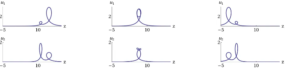
Figure 1. Parametric plots (with parameter ¯x) of the two componentsu1andu2for a 2-soliton solution of the 2-component short pulse equation (5.11) withǫ=−1, determined by the data of Example1 with
N = 2,s1= 1, s2= 2 andC= diag(1 + 3i,1−3i,2 + i/2,2−i/2) atx=−3,−1,1.
Example 1. We can alternatively express the solution given in Proposition 6 in the a priori more redundant form
q =±UΞ In−ǫ(KΞ)˜ 2−1V, p=ǫUΞ˜KΞ˜ In−ǫ(KΞ)˜ 2−1V,
with
SK+KS =V U, Ξ =˜ CΞ,
where C is any constant n×nmatrix that commutes withS. More precisely, the introduction of C allows us to fix some of the freedom in the choice of the coefficients of the matricesU,V. The following choices involve further restrictions, however. We consider the casem= 2,n= 2N, and choose
S = diag(s1I2, . . . , sNI2), U = σ1 . . . σ1 , V =
I2
.. . I2
,
where σ1 is the respective Pauli matrix. The Sylvester equation is then solved by
Kij =
1 si+sj
σ1, i, j= 1, . . . , N.
Choosing C block-diagonal where the 2 ×2 blocks on the diagonal are a linear combination of I2 and the Pauli matrixσ3 = diag(1,−1), then C commutes withS. Furthermore, it follows
thatKΞ consists of 2˜ ×2 blocks (KΞ)˜ ij which are linear combinations of the off-diagonal Pauli
matrices σ1 and σ2. It further follows that ((KΞ)˜ 2)ij is diagonal. As a consequence, the inverse
ofI2N−ǫ(KΞ)˜ 2 also consists of diagonal 2×2 blocks11. BecauseU consists of off-diagonal 2×2
blocks, we conclude that q given by the above formula is an off-diagonal 2×2 matrix. Hence its square is proportional to the identity matrix I2. Since N ∈ Nis arbitrary, we thus have an
infinite family of exact solutions of the system (5.11) with r= 2, where the components of the vectoru= (u1, u2)⊺ are given byu=u1σ1+u2σ2. Fig. 1shows a plot of a 2-soliton solution.
Remark 7. In order to obtain a Lax pair for the short pulse equation, we start with
ψx=
L−ν 2I
ψ, ψx¯=
¯ L− 1
2νI
ψ,
11
with L and ¯L taken from Remarks 2 and 6, respectively. Without imposing a reduction, the integrability conditions are (5.4) and (5.5) (modulo an integration with respect to ¯x). Writing ψ(x,x¯) =χ(x, z(x,x¯)), we find symmetry u 7→ −u of the short pulse equation, we recover the Lax pair given in [36] for the scalar case and withǫ=−1.
6
Dual AKNS hierarchies
For the bidifferential calculus determined by (3.7), the Miura transformation (2.3) with ∆ = 0 takes the form
λ−1 g−g−[λ]g−1 =Pφ−φ−[λ]P, (6.1)
and thedual equation (2.4) becomes
µ−1 Pg−[µ]g−1−(g−[µ]g−1)−[λ]P
To order µ0 this yields
λ−1 g−1Pg−(g−1Pg)−[λ]
= (g−−[1λ]Pg)x. (6.3)
Applying a Miwa shift with −[µ] and subtracting the result from this equation, we obtain
µ−1g−−[1λ]Pg−(g−−1[λ]Pg)−[µ] integration”. Hence (6.2) reduces to (6.3). The first non-trivial equation resulting from an expansion of (6.3) in powers of the indeterminate λis obtained as the term linear inλ,
(g−1Pg)t2 −(g −1Pg)
xx =−2 (g−1)xPgx. (6.4)
6.1 Miura transformation and relation
with the generalized Heisenberg magnet model
Introducing
(see also [18]), we have the identities
The dual hierarchy equation (6.4) can now be expressed as follows,
St2 =Sxx+ 2 g −1g
x(I+S)x.
In order to express this solely in terms of S we use the Miura transformation (6.1), which to order λ0 reads
gxg−1 = [P, φ] =
1
2[J, φ]. (6.7)
This imposes the following condition on g,
Inserting this in the expression for St2, and using the above identities, leads to
St2 =Sxx−(SxS(I+S))x = 1
2[S,Sxx] = 2F
(1)
x , (6.10)
which is the (generalized) Heisenberg magnet equation (see also Remark 5).
Remark 8. The ordinary Heisenberg magnet equationS~t=S~×S~xx is obtained from the 2×2
matrix case by writing S = P3k=1Skσk, where σ1, σ2, σ3 are the Pauli matrices, and setting
t2 =−it.
More generally, with the help of the Miura transformation (6.1) the hierarchy equations resulting from (6.3) can be expressed solely in terms of S. (6.1) implies
λ−1J,(g−g−[λ])g−1 ={J,Pφ−φ−[λ]P}=
hence, using (6.6) and (6.9),
which likely extends to all higher n∈N. Of course, the expression for St
n can be recovered by inserting the corresponding expression for g−1g
tn in (6.5).
Remark 9. Conditions like (6.8)12 originated from the use of the Miura transformation, and they are in fact needed to express the original hierarchy for the matrix variableg in terms ofS. The “mismatch” in the Miura transformation, leading to the restriction of the form ofg, can be traced back to the fact that in the step from (2.4) to (2.3) we are dropping cohomological terms (see Remark 4).
and thus
S =g−1Jg = 1 κ¯κ−σσ¯
κκ¯+σσ¯ 2κσ
−2¯κσ¯ −κ¯κ−σσ¯
.
The condition (6.8) amounts to κxκ¯ −σxσ¯ = 0 and κ¯κx −σ¯σx = 0. By adding these two
equations, we find that
(κκ¯−σσ¯)x= 0. (6.14)
Remark 10. Using the Miura transformation (2.3), the linear equation (3.21) reads
¯
dΨ =(¯dg)g−1Ψ + 2zdΨ
(writing ν = 2z), hence
¯
d ˆψ= 2zd ˆψ+g−1(dg) ˆψ
in terms of
ˆ
ψ=g−1Ψ.
Evaluation of the linear equation for the bidifferential calculus given by (3.7) leads to
λ−1ψˆ−λ−1ψˆ−[λ](I−2zλP) = 2z g−−1[λ]Pg
ˆ
ψ.
Writing
ˆ
ψ=ψe−Pn≥1(2zP)ntn,
we obtain
λ−1(ψ−ψ−[λ]) = 2z g−−[1λ]Pg
ψ=z g−−[1λ]g(I+S)ψ.
Expansion in powers of λyields
ψx=z(I+S)ψ,
ψt2 =
2z2(I+S)−zSxS
ψ,
ψt3 =
h
4z3(I+S)−2z2SxS+
z
2 2Sxx+ 3Sx
2 Siψ,
ψt4 =
"
8z4(I+S)−4z3SxS+z2 2Sxx+ 3Sx2S
−z2 2SxxxS −2SxxSx−4SxSxx−5Sx3S
#
ψ.
6.2 A class of solutions
The following result is an analog to that in Section 3.3 (see also Remark 3 in [1]). It allows to generate solutions of (2.4) from solutions of a linear system.
Theorem 2. Let (Ω,d,¯d) be a bidifferential calculus with Ω =A ⊗V(CN) andA= Matn0(B),
for some n0 ∈N. For f ixed n≥n0, let S∈Mat(n, n,B) and∆∈Mat(m, m,B). Furthermore, let X ∈Mat(n, n,B) andW ∈Mat(m, n,B) satisfy the linear equations
¯
dX = (dX)S, d¯W = (dW)S,
and also
XS−RX = ˜V Z, W S−∆W =CX, (6.15)
with matrices C,Z ∈Mat(m, n,B), R∈Mat(n, n,B) and V˜ ∈Mat(n, m,B), satisfying
dC = 0, dR= 0, d ˜V = 0, ¯d ˜V = 0.
Then
g= W X−1V˜−1, (6.16)
provided the inverse exists, solves the (modified) Miura transformation equation (2.3), i.e.
[¯dg−(dg)∆]g−1 = dφ, (6.17)
with some m×m matrix φ, and thus(by application ofd) also (2.4), i.e.13
d ¯dg−(dg)∆g−1= 0. (6.18)
Proof . Using the Leibniz rule and the assumptions, we have
¯
dg−1= (¯dW)X−1V˜ −W X−1(¯dX)X−1V˜
= (dW)SX−1V˜ −W X−1(dX)SX−1V˜ = dW −W X−1dXSX−1V˜
= d W X−1XSX−1V˜ = d W SX−1V˜−W X−1d XSX−1V˜
= d ∆g−1−W X−1d(RX+ ˜V Z)X−1V˜= d ∆g−1−g−1d ZX−1V˜,
and thus
[¯dg−(dg)∆]g−1 = d ZX−1V˜ −g∆g−1.
Remark 11. The assumptions in Theorem 2 give rise to integrability conditions. The latter are satisfied if
¯
dS = (dS)S, ¯d∆ = (d∆)∆, d¯C = (d∆)C, ¯dZ= (dZ)S.
In the following we exploit Theorem2for the bidifferential calculus given by (3.7) with some simplifications. We set ∆ = 0 and make the further assumption thatS is d- and ¯d-constant, and we write Z = ˜U Y, where ˜U ∈Mat(m, n,B) is d- and ¯d-constant and Y ∈Mat(n, n,B) solves
13
¯
dY = (dY)S. This is motivated by the fact that then the first of conditions (6.15) reduces to (3.25), i.e.
SK−KS =V U, (6.19)
assuming that Ad is invertible and using results from Section 3.3, in particular the defini-tions (3.26) for K,U,V. Furthermore, we obtain
W =Wd+WoΞ, Ξ=e−ξ(S)J, ξ(S) =
X
k≥1 Sktk,
and the second of conditions (6.15) yields C = WdSA−d1 (which simply determines C) and,
assuming that S is invertible,
Wo=−WdSKS−1.
The solution (6.16) of (6.18) (with ∆ = 0) is then given by
g−1 =W
d I−SKS−1Ξ(I−KΞ)−1V.
Rewriting this as
g−1 =Wd I−SKS−1Ξ
(I+KΞ) I−(KΞ)2−1V
=Wd I−SKS−1Ξ−SKS−1ΞKΞ+KΞ I −(KΞ)2−1V,
it can easily be decomposed into a part that commutes withJ,
g−1d=Wd I−SKS−1ΞKΞ I−(KΞ)2−1V
=WdV +Wd(KS−SK)S−1ΞKΞ I−(KΞ)2−1V
=WdVI−U S−1ΞKΞ I−(KΞ)2−1V,
and a part that anti-commutes with J,
g−1
o=Wd(KS−SK)S
−1Ξ I −(KΞ)2−1 V
=−WdV U S−1Ξ I −(KΞ)2−1V.
Using our concrete form of J and J, the matrices K, S, U, V have the form given in (3.32), and we have
Wd=
W 0
0 W¯
, Ξ=
Ξ 0 0 Ξ¯
, Ξ =e−ξ(S), Ξ =¯ eξ(−S¯).
This leads to
g−1 =
κ −σ
−¯σ κ¯
where
κ= (W V)I+US¯−1Ξ ¯¯KΞ(I−KΞ ¯¯KΞ)−1V, ¯
κ= ( ¯WV¯)I+ ¯U S−1ΞKΞ(¯ I−K¯ΞKΞ)¯ −1V¯, σ =−(W V)US¯−1Ξ(¯ I −K¯ΞKΞ)¯ −1V ,¯
¯
The only restrictions that have to be imposed on the matrices K, ¯K,S, ¯S,U, ¯U, V, ¯V result from (6.19). They are
SK+KS¯=V U, S¯K¯ + ¯KS = ¯VU .¯ (6.20)
The solutions of the hierarchy forgobtained in this way also determine solutions of the generali-zed Heisenberg hierarchy. This is so because the solutions constructed above via Theorem 2are actually solutions of the Miura transformation and our choice of matrix data via Proposition1
ensures that (3.14) holds (which we used in Section6.1).
6.3 Reciprocal dual and combined dual AKNS hierarchies
Elaborating the dual equation (2.4) with the “reciprocal” bidifferential calculus determined by (4.1), instead of using that determined by (3.7), we simply obtain (6.2) with g replaced byg−1. Again, we can combine the dual AKNS hierarchy and its reciprocal version, adopting the
procedure in Section 5. New equations arise from the mixed parts, hence from evaluating (2.4) using the bidifferential calculus given by
df = [PEλ, f]ζ+µ−1[¯Eµ, f]¯ζ, d¯f =λ−1[Eλ, f]ζ+ [PE¯µ, f]¯ζ,
which is a constituent of the calculus determined by (5.1). This results in
Pg−[µ¯]Pg−1− g−[¯µ]Pg−1−[λ]P−µ−1λ−1g−[λ]g−1− g−[λ]g−1
−[µ¯]
= 0.
To order λ0µ0 this is
gxg−1x¯+P, gPg−1= 0,
hence
gxg−1x¯ = 1
4 g˜g
−1
−gg˜ −1 where ˜g=JgJ. (6.21)
The Miura transformation between the combined hierarchies consists of a pair of Miura transformations, one for the original hierarchy and another one for the reciprocal. It results in the following two generating equations,
λ−1 g−g−[λ]
g−1 =Pφ−φ−[λ]P, Pg−g−[λ¯]P
g−1 =λ−1 φ−φ−[λ¯].
In particular, this yields
gxg−1 = [P, φ], φ¯x= [P, g]g−1. (6.22)
The formulas in Section6.2still generate solutions of the combined dual hierarchy and also of the Miura transformation (cf. (6.17)), provided we extend the expression forξ(S) used there to
ξ(S) =X
k≥1
Sktk+
X
k≥1
6.3.1 Sine-Gordon solutions
If m= 2 and ifg has the form
g=f
cos(ϑ/2) −sin(ϑ/2) sin(ϑ/2) cos(ϑ/2)
=f eIϑ/2, I=
0 −1
1 0
,
where f is a function independent ofx, then (6.21) becomes the sine-Gordon equation
ϑxx¯= sin(ϑ).
The function f drops out of equation (6.21). As a consequence of the form of g, the condi-tion (6.8), which arose from the Miura transformation, is satisfied. (6.22) requires the reduction conditions (5.6) withǫ=−1 and then reads
q =−1
2ϑx, qx¯ =− 1
2sin(ϑ), px¯= 1
2[1−cos(ϑ)].
In order to generate solutions of the sine-Gordon equation (and more generally of the cor-responding hierarchy), we have to choose the matrix data in such a way that g has the above form. We set
¯
K =−K, S¯=S, U¯ =−U, V¯ =V, W¯ =W.
Then (6.20) reduces to a single Sylvester equation, SK +KS = V U. Setting t2k = ¯t2k = 0,
k= 1,2, . . ., (6.23) has the property ξ(−S) =−ξ(S). As a consequence, we have ¯Ξ =eξ(−S) =
e−ξ(S)= Ξ and thus
κ= ¯κ=αI−U S−1ΞKΞ I+ (KΞ)2−1V, σ=−σ¯ =−αU S−1Ξ I+ (KΞ)2−1V,
whereα =W V. We still have to ensure thatκ2+σ2 =f2, with some functionf that does not depend on x. But since our procedure actually solves the Miura transformation (recall (6.17)), we already know that (6.8) is satisfied, hence (6.14) holds, which shows thatκ2+σ2 indeed does not depend on x.
Example 3. Let n = 1, S = s ∈ R, and U = V = W = 1. Then the Sylvester equation SK+KS =V U is solved by K = 21s. Writing Ξ = 2se−ξ˜(s), where ˜ξ(s) =P
k≥0(s2k+1t2k+1+
s−2k−1¯t
2k+1)+ξ0with a constantξ0, we obtainκ= tanh ˜ξ(s) andσ = sech ˜ξ(s), so thatκ2+σ2=1.
From σ/κ = csch ˜ξ(s) then follows the well-known kink solution ϑ = 2 arctan(csch ˜ξ(s)) = 4 arctaneξ˜(s). Withn >1 and real diagonal S we obtain multi-kink solutions.
7
Conclusions
We have shown in particular how a large family of solutions of matrix NLS equations, obtained in [2] with the help of general results of [1], extends to solutions of the corresponding hierarchies. Moreover, by a simple exchange of the roles of d and ¯d, we obtained a “reciprocal” or “purely negative” counterpart of the AKNS hierarchy, which turned out to be the nonlinear part of the potential KP hierarchy. Combining the two hierarchies then gives rise to additional “mixed flows”. In this way we recovered in particular the short pulse equation and obtained an apparently new vector version of it (different from those considered in [42, 44]), for which we presented soliton solutions in the 2-component case.
generalized Heisenberg magnet model. As the first “mixed flow” of the dual hierarchy combined with its negative counterpart, with a certain reduction the sine-Gordon equation showed up.
In this work we concentrated on a simple method, introduced in [1], to generate a class of so-lutions, parametrized by certain matrix data (essentially of arbitrary size) subject to a Sylvester equation. The largest part of the work in [2] concentrated on narrowing down a remaining redundancy in the matrix data that determine a matrix NLS solution. We expect that most of these results can be carried over to the cases treated in the present work.
Acknowledgements
We would like to thank Sergei Sakovich and some anonymous referees for helpful comments.
References
[1] Dimakis A., M¨uller-Hoissen F., Bidifferential graded algebras and integrable systems,Discrete Contin. Dyn. Syst. Suppl.2009(2009), 208–219,arXiv:0805.4553.
[2] Dimakis A., M¨uller-Hoissen F., Solutions of matrix NLS systems and their discretisations: a unified treat-ment,Inverse Problems26(2010), 095007, 55 pages,arXiv:1001.0133.
[3] Nijhoff F.W., Linear integral transformations and hierarchies of integrable nonlinear evolution equations,
Phys. D31(1988), 339–388.
[4] Fuchssteiner B., Fokas A.S., Symplectic structures, their B¨acklund transformations and hereditary symmet-ries,Phys. D4(1981), 47–66.
[5] Verovsky J.M., Negative powers of Olver recursion operators,J. Math. Phys.32(1991), 1733–1736.
[6] Tracy C.A., Widom H., Fredholm determinants and the mKdV/sinh-Gordon hierarchies, Comm. Math. Phys.179(1996), 1–9,solv-int/9506006.
[7] Ji J., Zhang J.-B., Zhang D.-J., Soliton solutions for a negative order AKNS equation hierarchy,Commun. Theor. Phys.52(2009), 395–397.
[8] Dorfmeister J., Gradl H., Szmigielski J., Systems of PDEs obtained from factorization in loop groups,Acta Appl. Math.53(1998), 1–58,solv-int/9801009.
[9] Kamchatnov A.M., Pavlov M.V., On generating functions in the AKNS hierarchy,Phys. Lett. A301(2002),
269–274,nlin.SI/0208025.
[10] Aratyn H., Ferreira L.A., Gomes J.F., Zimerman A.H., The complex sine-Gordon equation as a symmetry flow of the AKNS hierarchy,J. Phys. A: Math. Gen.33(2000), L331–L337,nlin.SI/0007002.
[11] Aratyn H., Gomes J.F., Zimerman A.H., On negative flows of the AKNS hierarchy and a class of defor-mations of a bihamiltonian structure of hydrodynamic type,J. Phys. A: Math. Gen.39(2006), 1099–1114, nlin.SI/0507062.
[12] Hasimoto H., A soliton on a vortex filament,J. Fluid Mech.51(1972), 477–485.
[13] Zakharov V.E., Takhtadzhyan L.A., Equivalence of the nonlinear Schr¨odinger equation and the equation of a Heisenberg ferromagnet,Theoret. and Math. Phys.38(1979), 17–23.
[14] Ishimori Y., A relationship between the Ablowitz–Kaup–Newell–Segur and Wadati–Konno–Ichikawa schemes of the inverse scattering method,J. Phys. Soc. Japan51(1982), 3036–3041.
[15] Wadati M., Sogo K., Gauge transformations in soliton theory,J. Phys. Soc. Japan52(1983), 394–398.
[16] Tsuchida T., Wadati M., Multi-field integrable systems related to WKI-type eigenvalue problems,J. Phys. Soc. Japan68(1999), 2241–2245,solv-int/9907018.
[17] Faddeev L.D., Takhtajan L.A., Hamiltonian methods in the theory of solitons, Springer Series in Soviet Mathematics, Springer-Verlag, Berlin, 1987.
[18] van der Linden J., Capel H.W., Nijhoff F.W., Linear integral equations and multicomponent nonlinear integrable systems. II,Phys. A160(1989), 235–273.
[20] Zakharov V.E., Shabat A.B., A scheme for integrating the nonlinear equations of mathematical physics by the method of the inverse scattering problem. I,Funct. Anal. Appl.8(1974), 226–235.
[21] Zakharov V., The inverse scattering method, in Solitons, Editors R. Bullough and P. Caudrey, Topics in Current Physics, Vol. 17, Springer, Berlin, 1980, 243–285.
[22] Konopelchenko B.G., On the structure of integrable evolution equations,Phys. Lett. A79(1980), 39–43.
[23] Gerdjikov V.S., Grahovski G.G., Kostov N.A., Multicomponent NLS-type equations on symmetric spaces and their reductions,Theoret. and Math. Phys.144(2005), 1147–1156.
[24] Gerdjikov V.S., Grahovski G.G., Multi-component NLS models on symmetric spaces: spectral properties versus representation theory,SIGMA6(2010), 044, 29 pages,arXiv:1006.0301.
[25] Dimakis A., M¨uller-Hoissen F., Functional representations of integrable hierarchies,J. Phys. A: Math. Gen. 39(2006), 9169–9186,nlin.SI/0603018.
[26] Bogdanov L.V., Konopelchenko B.G., Analytic-bilinear approach to integrable hierarchies. II. Multicompo-nent KP and 2D Toda lattice hierarchies,J. Math. Phys.39(1998), 4701–4728,solv-int/9705009.
[27] Konopelchenko B., Strampp W., The AKNS hierarchy as symmetry constraint of the KP hierarchy,Inverse Problems7(1991), L17–L24.
[28] Athorne C., Fordy A., Generalised KdV and MKdV equations associated with symmetric spaces,J. Phys. A: Math. Gen.20(1987), 1377–1386.
[29] Horn R.A., Johnson C.R., Topics in matrix analysis, Cambridge University Press, Cambridge, 1991.
[30] Cherednik I., Basic methods of soliton theory, Advanced Series in Mathematical Physics, Vol. 25, World Scientific Publishing Co., Inc., River Edge, NJ, 1996.
[31] Golubchik I.Z., Sokolov V.V., Generalized Heisenberg equations on Z-graded Lie algebras, Theoret. and Math. Phys.120(1999), 1019–1025.
[32] Rabelo M., On equations which describe pseudospherical surfaces,Stud. Appl. Math.81(1989), 221–248.
[33] Beals R., Rabelo M., Tenenblat K., B¨acklund transformations and inverse scattering solutions for some pseudospherical surface equations,Stud. Appl. Math.81(1989), 125–151.
[34] Sakovich A., Sakovich S., On transformations of the Rabelo equations, SIGMA 3 (2007), 086, 8 pages, arXiv:0705.2889.
[35] Sch¨afer T., Wayne C.E., Propagation of ultra-short optical pulses in cubic nonlinear media,Phys. D 196
(2004), 90–105.
[36] Sakovich A., Sakovich S., The short pulse equation is integrable, J. Phys. Soc. Japan74(2005), 239–241, nlin.SI/0409034.
[37] Sakovich A., Sakovich S., Solitary wave solutions of the short pulse equation, J. Phys. A: Math. Gen.39
(2006), L361–L367,nlin.SI/0601019.
[38] Brunelli J.C., The bi-Hamiltonian structure of the short pulse equation,Phys. Lett. A353(2006), 475–478, nlin.SI/0601014.
[39] Kuetche V.K., Bouetou T.B., Kofane T.C., On two-loop soliton solution of the Sch¨afer–Wayne short-pulse equation using Hirota’s method and Hodnett–Moloney approach, J. Phys. Soc. Japan76(2007), 024004,
7 pages.
[40] Kuetche V.K., Bouetou T.B., Kofane T.C., On exact N-loop soliton solution to nonlinear coupled disper-sionless evolution equations,Phys. Lett. A372(2008), 665–669.
[41] Parkes E.J., Some periodic and solitary travelling-wave solutions of the short-pulse equation,Chaos Solitons Fractals38(2008), 154–159.
[42] Pietrzyk M., Kanattsikov I., Bandelow U., On the propagation of vector ultra-short pulses, J. Nonlinear Math. Phys.15(2008), 162–170.
[43] Matsuno Y., Soliton and periodic solutions of the short pulse model equation,arXiv:0912.2576.