El e c t ro n ic
Jo ur
n a l o
f P
r o
b a b il i t y
Vol. 15 (2010), Paper no. 36, pages 1143–1160. Journal URL
http://www.math.washington.edu/~ejpecp/
Entropy of random walk range on uniformly transient and
on uniformly recurrent graphs
David Windisch
The Weizmann Institute of Science Faculty of Mathematics and Computer Science
POB 26 Rehovot 76100
Israel
Abstract
We study the entropy of the distribution of the setRnof vertices visited by a simple random walk on a graph with bounded degrees in its firstnsteps. It is shown that this quantity grows linearly in the expected size ofRnif the graph is uniformly transient, and sublinearly in the expected size if the graph is uniformly recurrent with subexponential volume growth. This in particular answers a question asked by Benjamini, Kozma, Yadin and Yehudayoff[1].
Key words:random walk, range, entropy.
AMS 2000 Subject Classification:Primary 60G50; 60J05.
1
Introduction
Let (Xn)n≥0 be a simple random walk on a graph G = (V,E) starting at some vertex o ∈ V. The entropy of the distribution of Xn for large nhas been studied on Cayley graphs and is known to be related to other objects of interest, such as the rate of escape and the existence of non-trivial bounded harmonic functions, see[5], [6], [10]. This work is devoted to the entropy of a similar observable, to that of the range of the random walk. LetRn={X0,X1, . . . ,Xn}be the set of vertices visited by the random walk in its firstnsteps. The entropy ofRnis defined as
Ho(Rn) =Eo
log
1
po(Rn)
, (1.1)
where the random walk starts at o ∈V, Po-a.s., po(A) = Po[Rn = A]for any finite connected set
A⊆ V containing o, and 0 log(1/0)is defined to be 0 as usual. According to Shannon’s noiseless coding theorem[9],Ho(Rn)/log 2 can be interpreted as the approximate number of 0-1-bits required per realization in order to encode a large number of independent realizations ofRn with negligible probability of error. Up to an additive constant, Ho(Rn)/log 2 can also be viewed as the expected
number of bits necessary and sufficient to encodeRn(see[3], Theorem 5.4.1), and as the expected number of fair coin tosses required for the simulation ofRn (see[3], Theorem 5.12.3).
The entropy ofRn for random walk on Zd, d ≥ 1, is investigated in a recent work by Benjamini,
Kozma, Yadin and Yehudayoff[1]. There, the authors show that the largenbehavior ofHo(Rn)is of ordernford≥3, of ordern/log2nford=2 and of order lognford=1. Comparing this behavior with that of the expected size〈Rn〉oofRn,
〈Rn〉o=Eo[|Rn|], (1.2)
known to be of ordernfor d ≥3, of order n/lognford = 2 and of orderpnford =1 (cf.[8], p. 221) , we observe that on Zd, H
o(Rn) grows linearly in 〈Rn〉o in the transient case and only
sublinearly in the recurrent case. On general graphs with bounded degrees, Ho(Rn) can grow at
most linearly in〈Rn〉o(see Proposition 2.4), but the assumptions on recurrence and transience alone do not allow us to conclusively compare Ho(Rn)with〈Rn〉o. Under slightly stronger assumptions, however, we can generalize the observation just made forZd to large classes of graphs.
The graphs we consider in this work are characterized by strengthened transience and recurrence conditions. Recall that a graph is transient if the escape probability Po[o∈ {/ X1,X2, . . .}]is strictly positive for any starting vertex o ∈ V. We call a graph G uniformly transientif such an estimate holds uniformly ino, that is, if
inf
o∈VPo[o∈ {/ X1,X2, . . .}]>0. (1.3)
Theorem 1.1 shows thatHo(Rn)grows linearly in〈Rn〉oon uniformly transient graphs with bounded
degrees. Such a statement does not hold under the assumption of transience alone, see Remark 3.5 for a counterexample.
Theorem 1.1. Let G be a uniformly transient graph with bounded degrees. Then
lim inf
n→∞ oinf∈V
Ho(Rn)
On the other hand, we call a graphG uniformly recurrentif sup
o∈V
Po[o∈ {/ X1, . . . ,Xn}]−→0, asn→ ∞. (1.5)
In addition, let|∂eB(x,r)| be the number of vertices at distance r+1 from x ∈V with respect to the usual graph distance. If the degrees of the graph are bounded byd≥2, then|∂eB(x,r)| ≤dr+1. The following condition requires slightly more:
for anyε >0, sup
x∈V|
∂eB(x,r)| ≤eεr, for infinitely manyr∈N. (1.6)
Under these conditions, we prove thatHo(Rn)grows only sublinearly in〈Rn〉o. We note that
recur-rence alone does not imply such a statement, see Remark 4.1 and also Remark 5.4.
Theorem 1.2. Let G be any uniformly recurrent graph with bounded degrees satisfying(1.6). Then
sup
o∈V
Ho(Rn)
〈Rn〉o −→0, as n→ ∞. (1.7)
The above results apply in particular to all vertex-transitive graphs. Recall that a graphG is vertex-transitive, if for every pair of vertices(x,x′), there is a bijectionφfromV toV such thatφ(x) =x′
andd(y,y′) =d(φ(y),φ(y′))for all y,y′∈V, whered(., .)denotes the usual graph distance. For vertex-transitive graphs, Ho(Rn) and〈Rn〉o do not depend on the starting vertex o of the random
walk, so we omit o from the notation. We can deduce the following dichotomy from the results above:
Theorem 1.3. Let G be a vertex-transitive graph.
If G is transient, then lim inf
n→∞
H(Rn)
〈Rn〉 >0, (1.8)
if G is recurrent, then H(Rn)
〈Rn〉 −→0, as n→ ∞. (1.9)
For uniformly transient graphs, 〈Rn〉 grows linearly in n (see Proposition 5.2). Hence, (1.8) in
particular shows thatH(Rn) grows linearly innon all vertex-transitive and transient graphs, thus answering a question asked in[1], Section 3.3.
We now comment on the proofs, starting with the one of Theorem 1.1, given in Section 3. A simple observation made in[1]shows thatHo(Rn)is bounded from below by a constant times the expected size of the interior boundary∂iRn ofRn. It thus suffices to prove a lower bound of order 〈Rn〉o on
Eo[|∂iRn|], or, equivalently, to prove that the fraction of the visited vertices belonging to ∂iRn is
non-degenerate probability that the walk then escapes from the ball B(x, 1) of radius 1 around it and leaves x in∂iRn. This yields the lower bound on Eo[|∂iRn|]required to prove Theorem 1.1. In
order to show that transience alone is not a sufficient assumption for the conclusion of Theorem 1.1, we consider a binary tree, where every edge at depth l is replaced by a path of length l+3, and show that this graph satisfies (1.7), see Remark 3.5 and Figure 1.
In the proof of Theorem 1.2 in Section 4, we cover every possible realization of Rn with one of at most supx∈V|∂eB(x,r)|(const.)|Rn|/r different collections of balls of radius r≥1. Uniform recurrence implies that most of these balls are typically completely covered byRn. We then consider the condi-tional entropy ofRn, given the numberK of such balls intersected byRn and the number Lof balls that are not completely filled byRn(the definition of conditional entropy is recalled in (2.4) below).
The conditional entropy can then be bounded by the expected logarithm of the number of possible configurationsRn can belong to, given(K,L) (cf. (2.7)). By assumption (1.6), the expected loga-rithm of the number of possible collections of covering balls can be made smaller thanε〈Rn〉ofor any
fixedε >0 by choosingr appropriately, while the assumption of uniform recurrence yields a similar bound on the expected logarithm of the number of possible choices of the exact configurations of
Rn in the few unfilled balls. This argument proves the required estimate on the conditional entropy
ofRn given(K,L). Since the entropy of(K,L)itself is only of order at most logn, this is sufficient for Theorem 1.2. Theorem 1.2 cannot be proved for every recurrent graph. As a counterexample, we consider a sequence of finite binary trees with rapidly increasing depths, connected together by a half-infinite path, see Remark 4.1 and Figure 2.
The article is organized as follows: In Section 2, we introduce notation and preliminary results on entropy, derive a general lower bound on 〈Rn〉o and show that Ho(Rn) grows at most linearly in
〈Rn〉o. Section 3 contains the proof of Theorem 1.1 and Section 4 proves Theorem 1.2. Finally, the
dichotomy for vertex-transitive graphs in Theorem 1.3 is deduced in Section 5.
Acknowledgement. The author is grateful to Itai Benjamini for helpful conversations and to an
anonymous referee for helpful remarks.
2
Notation and preliminaries
In this section, we introduce the notation and prove some preliminary results. These include a lower bound of order pn on the expected size ofRn on a general infinite graph with bounded degrees,
obtained in Proposition 2.3 by adapting an argument in[7], as well as the observation thatHo(Rn)
grows at most as fast as the expected size 〈Rn〉o on any infinite connected graph with bounded degrees.
Throughout this article, we let G = (V,E)be a graph. V denotes the set of vertices and E the set of edges consisting of unordered pairs of vertices inV. Whenever{x,y} ∈ E, we write x ∼ y and call the vertices x and y neighbors. The number of neighbors of a vertex x is always assumed to be finite and referred to as the degree of x, denoted deg(x). A path of length l is a sequence
graphG has bounded degrees if supx∈Vdeg(x) ≤d for somed ≥1. For any setAof vertices, we define the interior and exterior boundaries of Aby∂iA={x ∈A: x ∼ y for some y ∈V \A}and ∂eA=∂i(V\A). The subgraph G(A) = (A,E(A))induced byA⊆ V consists of the vertices inAand the set of edgesE(A) ={{x,y} ∈E:{x,y} ⊆A}. We say thatAis connected ifG(A)is connected in the above sense. The cardinality of any setAis denoted by|A|, the largest integer less thana∈Rby
[a]and the minimum of numbersa,b∈Rbya∧b. Throughout the text,corc′are used to denote strictly positive constants with values changing from place to place. Dependence of constants on additional parameters appears in the notation. For example,cd denotes a positive constant possibly
depending ond.
For any x ∈V, we denote byPx the law onVN (equipped with the canonicalσ-algebra generated by the coordinate projections) of the Markov chain onV starting at x with transition probability
p(x,y) =
¨
1/deg(x), if x∼ y,
0, otherwise,
and write (Xn)n≥0 for the canonical coordinate process, referred to as the simple random walk on
G. The corresponding expectation is denoted by Ex, the canonical shift-operators onVNby(θn)n≥0. Note that deg(x)p(x,y) =deg(y)p(y,x), meaning that the measureπ:A7→Px∈Adeg(x)on V is a reversible measure for the simple random walk. The first entrance and hitting times of a setAof vertices are defined as
τA=inf{n≥0 :Xn∈A},τ+A =inf{n≥1 :Xn∈A}, (2.1) where we write τx rather than τ{x} if Aconsists of a single element x. The capacity of a finite nonempty subsetAofV is defined as
cap(A) =X
x∈A
Px[τ+A =∞]deg(x). (2.2)
We will generally refer to the starting vertex of the random walk aso. It will be convenient to define the collectionCoas
Co={A⊆V :Ais finite, connected, ando∈A}. (2.3)
Note thatRn ∈ Co, Po-a.s. The entropy of the rangeRn of the random walk has been defined in (1.1). More generally, for any random variableX taking values in a countable setX, we define the entropy ofX by
Ho(X) =Eo
log
1
po(X)
, where po(x) =Po[X =x], for x ∈ X.
Given another random variableY taking values in a countable setY, the conditional entropy ofX
givenY is defined by
Ho(X|Y) =Ho (X,Y)
−Ho(Y). (2.4)
An application of Jensen’s inequality shows that
while the following estimate is elementary:
Ho(X)≤Ho(X|Y) +Ho(Y). (2.6) Moreover, we have the following useful lemma:
Lemma 2.1. For random variables X and Y with values in countable setsX andY,
Ho(X|Y)≤Eo[log|XY|], where (2.7)
The following simple lemma, combined with a covering argument, will be instrumental in proving the bound onHo(Rn)in Theorem 1.2.
Lemma 2.2. Let G = (V,E) be any graph with bounded degrees, o ∈V , and let A∈ Co (cf.(2.3)). Then there exists a nearest-neighbor path in G(A)starting at o, covering A, and of length at most2|A|. Proof. The standard depth-first search algorithm (see [2]) yields a spanning tree TA = (A,ET) of
G(A) (i.e. a tree with vertices Aand edges ET ⊆ E(A)), as well as a nearest-neighbor path in TA
coveringAand traversing every edge inET at most once in every direction. Since the length of such a path is bounded from above by 2|ET|=2(|A| −1)<2|A|, the statement follows.
We now prove a general lower bound on the expected range of random walk on an infinite connected graph with bounded degrees. This lemma will allow us to disregard small errors when relating
Ho(Rn)to〈Rn〉o.
Proposition 2.3. Let G= (V,E)be any infinite connected graph with bounded degrees. Then
lim inf
n→∞ oinf∈V
〈Rn〉o
p
n >0. (2.8)
Proof. This proof is an adaptation of an argument appearing in[7]in the context of random walk on Cayley graphs. Let(Nk)k≥1 be the successive times when the random walk visits a new vertex, that is,N1=0, and fork≥1,Nk=inf{n>Nk−1:Xn∈ {/ X0, . . .XN
k−1}}. Then we have fork≥1 and
o∈V, by the Chebychev inequality,
Noting thatXl6=XN
i forl<Ni and applying the strong Markov property at timeNi, we deduce that Po[|Rn| ≤k]≤ k
n X
0≤l≤n
sup
x∈V
Px[Xl=x].
By a general heat-kernel upper bound, we have supx,y∈VPx[Xl= y]≤cd/
p
l+1, for some constant
cd > 0 depending on the uniform bound d on degrees (see, for example, [11], Corollary 14.6, p. 149). Hence, we find
Po[|Rn| ≤k]≤cdpk
n, fork≥1.
This last inequality, applied withk= [pn/(2cd)], yields
Eo[|Rn|]≥
p
n
2cd
Po[|Rn|>[pn/(2cd)]]≥
p
n
4cd
.
Finally, we prove that on any infinite connected graph with bounded degrees,Ho(Rn)does not grow faster than〈Rn〉o.
Proposition 2.4. Let G= (V,E)be any infinite connected graph with degrees bounded by d. Then
lim sup
n→∞ sup
o∈V
Ho(Rn)
〈Rn〉o ≤
2 logd.
Proof. Lemma 2.1 and Lemma 2.2 together imply that
Ho(Rn||Rn|)≤ 〈Rn〉o2 logd, whereas it follows from (2.5) that
Ho(|Rn|)≤log(n+1).
Hence by (2.6),Ho(Rn)≤ 〈Rn〉o2 logd+log(n+1). Proposition 2.3 completes the proof.
3
The transient case
In this section, we prove Theorem 1.1 asserting that the entropy ofRn grows at least linearly in its
expected size〈Rn〉oon any uniformly transient graph.
Lemma 3.1 and Corollary 3.2 show thatHo(Rn)grows at least linearly in the expected size〈∂iRn〉o
of∂iRn. These two statements and their proofs are straightforward adaptations of Lemma 3 and Corollary 4 in[1].
Lemma 3.1. For any graph G with degrees bounded by d≥2,
Proof. Fix A ⊆ V and define the successive entrance times to ∂iA by T1 = τ∂
Corollary 3.2. For any graph G with degrees bounded by d≥2, Ho(Rn)≥(〈∂iRn〉o−1)log (1−d−1)−1 will eventually prove that many vertices of degree at least 3 typically belong to∂iRn. To this end,
we prove in the following lemma that such vertices exist within constant distance of any vertex in uniformly transient graphs. For notational convenience, we introduce the parameter
α= inf
x∈VPx[τ
+
x =∞], (3.3)
which is strictly positive ifGis uniformly transient (cf. (1.3)).
Lemma 3.3. Let G be a uniformly transient graph withα as in(3.3). Then for any x ∈V , there is a side of (3.4) equals 0. Otherwise, the escape probability is equal to the probability that a simple random walk onZstarted at 1 reaches r before 0, hence to 1/r (see, for example,[4], Chapter 3, Example 1.5, p. 179). It follows thatα≤1/r.
Lemma 3.4. Let G be a uniformly transient graph. Then
inf
A⊆V,A6=;cap(A)≥α. (3.5)
Proof. By uniform transience, cap({x}) ≥ αdeg(x) ≥ α for all x ∈ V (see (1.3)). The statement (3.5) thus follows immediately from monotonicity of cap:
for finite, non-empty setsA⊆B⊆V, cap(A)≤cap(B). (3.6) Here is a direct proof of this well-known property: by summing over all possible timesnand loca-tions y of the last visit of the random walk to the set B and using the simple Markov property at timen, we find that, forA,Bas above,
cap(A) = X
x∈∂iA ∞
X
n=0
X
y∈∂iB
Px[τ+A >n,Xn= y,τ+B ◦θn=∞]deg(x) (3.7)
= X
x∈∂iA ∞
X
n=0
X
y∈∂iB
Px[τ+A >n,Xn= y]Py[τ+B =∞]deg(x).
Reversibility of the simple random walk implies that
deg(x)Px[τA+>n,Xn=y] =deg(y)Py[τA=n,Xn=x], hence by (3.7) that
cap(A) = X
y∈∂iB
deg(y)Py[τA<∞]Py[τ+B =∞]≤cap(B),
proving (3.6).
We now come to the main objective of this section.
Proof of Theorem 1.1. We will prove that
lim inf
n→∞ oinf∈V
〈∂iRn〉o
〈Rn〉o
>0. (3.8)
The desired statement then follows by Corollary 3.2 and the fact that inf
o∈V〈Rn〉o→ ∞,
proved in Proposition 2.3 (indeed, all connected components of a transient graph are infinite). Denote the set of vertices with degree at least 3 byV≥3 and the uniform bound on the degrees byd. Observe that any vertexx inV≥3 belongs to∂iRnif it is visited by the random walk, but at least one of its neighbors is not. Hence, for any x∈V≥3, the probability of{x ∈∂iRn}is bounded from below
B(x, 1)until timen. By the strong Markov property applied at timeτB(x,1)+2 and at timeτB(x,1),
where we have applied Lemma 3.4 with A = B(x, 1) in order to bound the escape probability
Pz[τ+B(x,1) = ∞] from below by α/d2. For any r ≥ 1, the random walk reaches B(x, 1) if it en-tersB(x,r)and then follows the shortest path toB(x, 1), hence,
Po[τB(x,1)≤n−2]≥Po[τB(x,r)≤n−1−r]d−(r−1). Using this estimate in (3.9), we obtain
〈∂iRn〉o≥ X
Remark 3.5. The conclusion (1.4) of Theorem 1.1 does not hold for every transient graph with
bounded degrees. For a counterexample, consider a binary tree Tb = (Vb,Eb) and denote bySl =
b}. Then elementary computations using the simple Markov property at time 1 (cf.[4], Chapter 4, Example 7.1, p. 271-272) show that for any vertexx inSl,
Hence, the process (Xσk)k≥1 is transient. In particular, the stretched graph G remains transient. Denote byR′n=Rn∩Vbthe intersection ofRnwith the vertices in the original tree. Then from (2.6), we obtain that
S1
S2 o
Figure 1: The stretched binary tree constructed in Remark 3.5. The filled vertices are the ones present in the original binary treeTb, the stretched treeGis obtained by adding the unfilled ones.
For any fixed realization of R′n of diameter m with respect to the original tree Tb, the set Rn is
determined up to the precise location of at most 2|R′n|boundary vertices on paths of length at most
m+3. Hence, for any such realization, there are at most(m+3)2|R′n|≤(c|R
n|)2|R
′
n|choices forRn. It therefore follows from Lemma 2.1 that
Ho(Rn|R′n)≤c Eo[|R′n|]logn.
The amount of time the process Xσ. spends in any given set Sk is by (3.11) and an elementary
estimate on biased random walk stochastically dominated by a geometrically distributed random variable with success probability 1/5 (cf. [4], Chapter 4, Example 7.1 (b), p. 271-272). It follows that
Eo[|R′n|]≤1+5Eo
X
1≤k≤n
1{τSk≤n}
(3.13)
≤c Eoh max
0≤k≤nd(o,Xk)
1/2i
≤c Eo[p|Rn|]. Applying Jensen’s inequality on the right-hand side, we deduce that
Ho(Rn|R′n)≤c〈Rn〉1o/2logn.
Regarding the other term on the right-hand side of (3.12), we have by the same argument as in the proof of Proposition 2.4,
Ho(R′n)≤c Eo[|R′n|]≤c〈Rn〉1o/2, by (3.13).
4
The recurrent case
In this section we prove Theorem 1.2, showing that supo∈VHo(Rn)/〈Rn〉o tends to zero as n→ ∞
on uniformly recurrent graphs satisfying the growth condition (1.6).
Recall that any realization of Rn belongs to Co, P-a.s. (cf. (2.3)). Our argument is based on
Lemma 2.2 showing that any set A ∈ Co can be explored by a path not longer than 2|A|. We
will use this fact in the proof of Theorem 1.2 in order to show that any realization of Rn can be covered by one of at most supx∈V|∂eB(x,r)|d|Rn|/rdifferent collections of balls of radiusr. The sec-ond key observation will be that due to uniform recurrence, most of these balls of radius r visited are typically completely covered by the random walk. This will show that the distribution ofRn is sufficiently concentrated to admit a bound onHo(Rn)sublinear in〈Rn〉o.
Proof of Theorem 1.2. We denote the uniform bound on degrees by d. Note that we can assume without loss of generality thatG is connected, for we may otherwise only consider the component of G containing the starting vertex o of the random walk. If G is finite, then (1.7) immediately follows from the fact that limnPo[Rn = V] = 1. Hence, we can from now on assume that G is
connected and infinite. In particular, Proposition 2.3 is available for application.
Consider anyo∈V andr≥1. For anyA∈ Co(cf. (2.3)), we define the finite sequence of vertices
Fr(A) = (x1, . . . ,xk) (4.1) such that the balls with radius r centered at x1, . . . ,xk cover A, trying to keepk as small as
pos-sible. We define Fk(A) inductively as follows: by Lemma 2.2, there is a nearest-neighbor path
pA= (p(0), . . . ,p(l))in G(A)starting ato=pA(0)and visiting all vertices inAinl ≤2|A|steps. Set
x1=o,t1=0, and fori≥2 such thatti−1<∞, define ti as
ti=
¨
inf{t >ti−1:pA(t)∈/B(xi−1,r)}, if ∪1≤j≤i−1B(xj,r)+A,
∞, otherwise,
and, providedti <∞, define xi= pA(ti). Since pAis of length at most 2|A|and covers all ofA, this yields a finite sequence as in (4.1), wherekis the largest index such thattk<∞and satisfies
k≤1+ [2|A|/r]. (4.2)
Finally, the construction implies that
∪ki=1B(xi,r)⊇A. (4.3)
We now partition the collectionCoaccording to the cardinality ofFr(A)and the number of verticesx
inFr(A)with the property thatB(x,r)is not completely filled byA: we haveCo=∪∞k=1∪kl=0C(k,l), where the disjoint collectionsC(k,l)are defined as
C(k,l) ={A∈ Co:|Fr(A)|=k,|{x ∈Fr(A):A+B(x,r)}|=l}. (4.4) We introduce the random variablesK andL, defined as
Observe that since|Rn| ≤n+1, (4.2) implies that
0≤L≤K≤[2(n+1)/r] +1, Po-a.s.
Using the elementary estimate (2.6) together with (2.5) and Lemma 2.1, we obtain the following bound on the entropy ofRn:
We now bound the number of choices we have when selecting a setAfrom the collectionC(k,l). For a set Ato belong to C(k,l), Fr(A) must consist of k vertices. The initial vertex x1 must be o
and each successive vertex must be at distance r+1 from the previous one. Hence, Fr(A)can take
at most skr different values. For every choice of Fr(A) = (x1, . . . ,xk), there are at most kl
≤ 2k
different choices of size-l subsets of vertices xi with the property that B(xi,r) is not completely filled byA. After selectingFr(A)and such a subset,Ais by (4.3) determined up to the at most(2br)l
possible configurations in the balls with centersxi that are not subsets ofA. Hence, we have log|C(k,l)| ≤k(logsr+log 2) +brllog 2. (4.8) Inserting this estimate into the above bound (4.6) onHo(Rn), we obtain
a
1a
2o
1o
2o
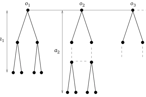
3Figure 2: The graph constructed in Remark 4.1.
we havePx[τy ≤τ+x]≥d−rfor any such y. With the strong Markov property applied at the times
Inserting the above estimates into (4.9), we deduce that
Ho(Rn)
Remark 4.1. The conclusion (1.7) of Theorem 1.2 does not hold for every recurrent graph with
bounded degrees, not even without the supremum over o∈V. As a counterexample, consider an infinite sequence of binary trees of finite depthsa1<a2<· · ·, with rootso=o1,o2, . . .. Regardless of the choice ofa1,a2, . . ., after addition of edges
{o1,o2},{o2,o3}, . . .
one obtains a connected and recurrent graph, illustrated in Figure 2. The sequence of depths can be chosen recursively such that
Po[τon≥
pa
(observe that the distribution of τo
n depends on a1, . . . ,an−1, but not on an). Denote the set of vertices in then-th tree at distancel fromon bySl, l ≥1. Observe that by an elementary estimate
on one-dimensional biased random walk, whenever the random walk reaches a previously unvisited levelSl at some vertexx ∈Sl, the probability that the random walk never returns toSl until time
an and thereby leaves x in ∂iRan is at least 1/3 (see, for example, [4], Chapter 4, Example 7.1,
using again an elementary estimate on one-dimensional biased random walk for the second in-equality. Hence, Corollary 3.2 shows thatHo(Rn)/〈Rn〉o does not tend to 0 for the recurrent graph
G defined above.
5
Vertex-transitive graphs
This final section contains the proof of Theorem 1.3 on the dichotomy for vertex-transitive graphs. Note that, due to vertex-transitivity, Ho(Rn), and 〈Rn〉o do not depend on o, so o can be omitted
from the notation. We first deduce the estimate in the recurrent case.
Corollary 5.1. Let G be any vertex-transitive and recurrent graph. Then
H(Rn)
〈Rn〉 −→
0, as n→ ∞. (5.1)
Proof. By Theorem 1.2, we only need to check conditions (1.5) and (1.6). Due to vertex-transitivity, the suprema become superfluous in both conditions. The assertion (1.5) is thus a consequence of recurrence and monotone convergence. Simple random walk on a vertex-transitive graph is quasi-homogeneous, see[11], Theorem 4.18, p. 47. As a consequence, if lim infr|B(o,r)|/r3 > 0, then
G satisfies a three-dimensional isoperimetric inequality, which implies in particular that the random walk is transient (we refer to[11], Corollary 4.16, p. 47, and Theorem 5.2, p. 49, for the proofs of these claims). Hence, we must have lim infr|B(o,r)|/r3 = 0, from which (1.6) immediately follows.
Proof of Theorem 1.3. Since the infimum in condition (1.3) is superfluous for vertex-transitive graphs, every vertex-transitive and transient graph is uniformly transient. Theorem 1.1 hence shows that
lim inf
n→∞ H(Rn)/〈Rn〉>0
in the transient case. Corollary 5.1 shows thatH(Rn)/〈Rn〉tends to 0 for vertex-transitive recurrent graphs. Since every vertex-transitive graph is either transient or recurrent, this proves Theorem 1.3.
In order to answer the question from [1] mentioned after Theorem 1.3, it remains to prove that
〈Rn〉 grows linearly in n for vertex-transitive transient graphs. This is surely well-known, but we could not find a proof in the literature, so we give a proof here. We denote the Green function of the simple random walk (evaluated on the diagonal) by
g(x) =Ex ∞
X
k=0
1{Xk=x}
, for x ∈V,
and the Green function of the random walk killed afternsteps by
gn(x) =Ex n
X
k=0
1{X
k=x}
, for x ∈V.
Proposition 5.2. Let G be any transient graph and let
e(x) =Px[τ+x =∞]∈(0, 1)
be the escape probability from vertex x∈V . Then
inf
o∈Ve(o)≤lim infn→∞ oinf∈V
〈Rn〉o
n . (5.2)
Moreover, if G is vertex-transitive and transient, then
〈Rn〉
n −→e(o)>0, as n→ ∞. (5.3)
Proof. LetG be any transient graph and o∈V. By the Markov property applied at time 1, g(x) =
1+ (1−e(x))g(x), hence
g(x) =1/e(x), for any x ∈V. (5.4)
Forn≥1 andx ∈V, we denote byNxn the total number of visits tox in the first nsteps,
Nxn= X
0≤k≤n
1{Xk=x}.
Summation over all vertices yields the total number of steps:
n+1=X
x∈V
Taking expectations in this equation and applying the strong Markov property at timeτx, we obtain that
n+1=X
x∈V
Eo[Nxn] (5.6)
≤X
x∈V
Po[τx ≤n]g(x)
≤ 〈Rn〉osup x∈V
g(x).
The estimate (5.2) is trivial if info∈Ve(o) =0 and follows from (5.4) and (5.6) otherwise.
Let nowG be a vertex-transitive transient graph. In particular, (5.2) holds without the infimum on either side. Replacingnby[λn]withλ >1 in (5.5), we have forn≥cλ,
[λn] +1≥X
x∈V
Eo[Nx[λn]1{τx≤n}]
≥X
x∈V
Po[τx ≤n]g[λn]−n(o)
=〈Rn〉og[λn]−n(o).
Lettingntend to infinity and using (5.4), it follows that for anyλ >1,
lim sup
n→∞
〈Rn〉o
n ≤λe(o).
We now letλtend to 1 and together with (5.2) obtain (5.3).
Remark 5.3. Theorem 1.1 and (5.2) prove that Ho(Rn)grows linearly innfor all uniformly tran-sient graphs with bounded degrees, while Theorem 1.2 in particular proves that Ho(Rn) grows sublinearly innon uniformly recurrent graphs satisfying the growth condition (1.6).
Remark 5.4. The example presented in Remark 4.1 does not satisfy the volume growth assumption
(1.6) and hence does not show that (1.6) is actually necessary in Theorem 1.2. We do not know of an example showing necessity of (1.6), or indeed if there even exists a graph satisfying (1.5) but not (1.6).
Remark 5.5. Given the results of the present work, it is natural to wonder whether one can
ob-tain more precise estimates on Ho(Rn) on vertex-transitive graphs or even prove an analogue of Shannon’s theorem on the almost-sure behavior of log(po(Rn)).
References
[1] I. Benjamini, G. Kozma, A. Yadin, A. Yehudayoff. Entropy of random walk range.
Ann. Inst. H. Poincaré Probab. Statist., to appear.
[3] T.M. Cover, J.A. Thomas. Elements of information theory.John Wiley & Sons, Inc., New York, 1991.
[4] R. Durrett.Probability: Theory and Examples.(third edition) Brooks/Cole, Belmont, 2005. [5] A. Erschler. On drift and entropy growth for random walks on groups. Ann. Probab. 31/3,
pp. 1193-1204, 2003.
[6] V.A. Ka˘ımanovich, A.M. Vershik. Random walks on discrete groups: boundary and entropy.
Ann. Probab., 11/3, pp. 457-490, 1983.
[7] A. Naor, Y. Peres. Embeddings of discrete groups and the speed of random walks.International Mathematics Research Notices2008, Art. ID rnn 076.
[8] P. Révész.Random walk in random and non-random environments. Second edition. World Sci-entific Publishing Co. Pte. Ltd., Singapore, 2005.
[9] C.E. Shannon. A mathematical theory of communication. The Bell System Technical Journal, Vol. 27, pp. 379-423, 623-656, 1948.
[10] N.T. Varopoulos. Long range estimates for Markov chains. Bull. Sci. Math. (2) 109, pp. 225-252, 1985.