Summary We derived a simplified version of a previously published process-based model of forest productivity and used it to gain information about the dependence of stemwood growth on nitrogen supply. The simplifications we made led to the following general expression for stemwood carbon (cw) as a function of stand age (t), which shows explicitly the main factors involved:
cw(t)=
ηwG∗
µw
1 −
λe−µwt−µ
we−λt
λ−µw
,
where ηw is the fraction of total carbon production (G) allo-cated to stemwood, G* is the equilibrium value of G at canopy closure, λ describes the rate at which G approaches G*, and µw is the combined specific rate of stemwood maintenance respi-ration and senescence. According to this equation, which de-scribes a sigmoidal growth curve, cw is zero initially and asymptotically approaches ηwG*/µw with the rate of approach dependent on λ and µw. We used this result to derive corre-sponding expressions for the maximum mean annual stem-wood volume increment (Y) and optimal rotation length (T). By calculating the quantities G* and λ (which characterize the variation of carbon production with stand age) as functions of the supply rate of plant-available nitrogen (Uo), we estimated the responses of Y and T to changes in Uo. For a plausible set of parameter values, as Uo increased from 50 to 150 kg N ha−1 year−1, Y increased approximately linearly from 8 to 25 m3 ha−1 year−1 (mainly as a result of increasing G*), whereas T decreased from 21 to 18 years (due to increasing λ). The sensitivity of Y and T to other model parameters was also investigated.
The analytical model provides a useful basis for examining the effects of changes in climate and nutrient supply on sus-tainable forest productivity, and may also help in interpreting the behavior of more complex process-based models of forest growth.
Keywords: canopy closure, mean annual increment, optimal rotation length, plantation, sustained yield.
Introduction
Quantifying the relationship between forest nutrition and for-est productivity is an important concern of plantation
manag-ers. Over the last decade, attempts to improve on yield predic-tions based on empirical site quality indices (e.g., Lewis et al. 1976) have led to the development of models based on the underlying biological processes that govern the relationship between productivity and nutrition (e.g., Dixon et al. 1990).
However, interpreting the behavior of biologically realistic models is often difficult because of the complexity of the processes involved. To facilitate such interpretation, and there-fore the translation of information from complex models to guidelines for forest practice, it is useful to examine the behav-ior of relatively simple process-based models that are amena-ble to analytical solution, even though quantitative accuracy is sacrificed to some extent for qualitative insight.
McMurtrie and Wolf (1983) and McMurtrie (1985, 1991) developed a process-based model of stand growth that simu-lates the effect of nitrogen supply on forest productivity. Re-cently, the model has been combined with the soil carbon--nitrogen model of Parton et al. (1987) and Schimel et al. (1990). The combined model (called G’DAY) has been used to examine the long-term response of unmanaged forest eco-systems to increasing CO2 concentration (Comins and McMurtrie 1993, Kirschbaum et al. 1994).
The aim of this study was to derive a simplified, analytically tractable version of the plant production part of G’DAY, and use it to gain insights into the general relationship between stemwood growth and nitrogen supply in managed forests. In particular, the model was used to predict how the maximum mean annual stemwood volume increment and optimal rota-tion length can be expected to vary in response to changes in the supply of nitrogen from net mineralization, fertilizer addi-tions, fixation and atmospheric deposition.
Simple stand growth model
Figure 1 shows the general structure of the model. Four dy-namic variables are represented: foliage carbon (cf, kg C m−2), foliage nitrogen (nf), stemwood carbon (cw, which includes stems, branches and coarse roots), and fine root carbon (cr). Table 1 lists the symbol definitions and units. A list of parame-ter values is given in Table 2. Some of these parameparame-ter values have been taken from Comins and McMurtrie (1993), others are biologically reasonable estimates. As such, the values have been chosen to illustrate the general behavior of the model, and do not reflect a particular species or data set.
Analytical model of stemwood growth in relation to nitrogen supply
RODERICK C. DEWAR and ROSS E. M
CMURTRIE
School of Biological Science, University of New South Wales, Sydney NSW 2052, Australia
Received March 2, 1995
The model equations are based on those of McMurtrie and Wolf (1983) and McMurtrie (1985, 1991):
dcf
dt =ηfG −γfcf (1a)
dnf
dt = U −(ηwνw+ηrνr)G −γfnf (1b)
dcw
dt =ηwG −(γw+ rw)cw (1c)
dcr
dt =ηrG −(γr+ rr)cr . (1d)
In Equation 1, carbon production (G, kg C m−2 year−1) is
allocated to foliage, stemwood and fine roots according to fixed allocation fractions ηi (i = f, w, r), with Σiηi = 1. Losses of carbon due to foliage, stemwood and fine root senescence occur at rates γi (i = f, w, r). Maintenance respiration in stemwood and fine roots (specific rates rw and rr, respectively) is also explicitly represented, whereas foliage maintenance respiration and all components of plant growth respiration are included implicitly in the definition of G. In Equation 1b, the rate of increase of foliage nitrogen is the balance between plant nitrogen uptake (U, kg N m−2 year−1), the allocation of nitrogen to stemwood and fine roots (derived from the respective carbon allocation fractions ηw and ηr and N/C ratios νw and νr, as-sumed constant), and the rate of return of nitrogen to the soil in leaf fall (for simplicity we ignored nitrogen retranslocation). Carbon production is assumed proportional to absorbed photosynthetically active radiation (φabs, GJ m−2 year−1):
G =εφabs. (2)
In the G’DAY model (Comins and McMurtrie 1993), the light utilization coefficient ε (kg C GJ−1 PAR) is assumed to be proportional to the foliage N/C ratio (νf = nf / cf) when nitrogen is limiting:
ε(νf)=εo
νf
νo
, if νf<νo (3a)
=εo, if νf≥νo (3b
where νo is the foliage N/C ratio below which carbon produc-tion is nitrogen-limited, and εo is the maximum value of ε obtained when nitrogen is non-limiting. Some other forms for
ε(νf) are considered by McMurtrie (1991); Equation 3 is adopted here for simplicity.
McMurtrie and Wolf (1983) and McMurtrie (1985, 1991)
Figure 1. General structure of the stand growth model, showing dy-namic variables (boxes), carbon fluxes (solid lines) and nitrogen fluxes (broken lines).
Table 1. Definition of symbols for main variables used (other symbols used in Appendices A−C are defined there). Abbreviations: units involving m−2 are per unit ground area; C = carbon; N = nitrogen; PAR = photosynthetically active radiation; X* = equilibrium value of X. Relevant equation numbers are given in square brackets. (See Table 2 for parameter definitions and values.)
Symbol Definition Units
cf, cf* Foliage C [1a, B6] kg C m−2
cr, cr* Fine root C [1d, B4] kg C m−2
cw, cw* Stemwood C [1c, 8, 9] kg C m−2
G, G* Total plant C production (net of canopy maintenance and plant growth respiration) [2, 7, B9] kg C m−2 year−1
nf Foliage N [1b] kg N m−2
t Stand age year
T Optimal rotation length [11, 12, 14a] year
U, U* Rate of N uptake by trees [5, B10] kg N m−2 year−1
Vw* Equilibrium stemwood volume [Table 3] m3 ha−1
Y Maximum mean annual stemwood volume increment [11, 13a, 14b] m3 ha−1 year−1
Yg Gross stemwood volume productivity at canopy closure [13b] m3 ha−1 year−1
ε Canopy light utilization coefficient [2, 3] kg C GJ−1 PAR
φabs PAR absorbed by the canopy [2, 4] GJ m−2 year−1
λ Rate of approach of G toward equilibrium [7, C5] year−1
µi, i = w and r Sum of maintenance respiration and senescence rates [10, B5] year−1
assumed a Beer’s law function for the relationship between φabs and foliage carbon. To make the model analytically tractable, we approximate Beer’s law using a hyperbolic function:
φabs(cf)=φo
cf
cf+ Kf
, (4a)
where φo is the amount of incident radiation at the top of the canopy, and Kf is the value of foliage carbon at which 50% of the incident light is absorbed. If k is the Beer’s law extinction coefficient and σ (m2 leaf kg−1 C) is the specific leaf area (i.e.,
φabs /φo = 1 − exp(−kσcf)), then matching Equation 4a to Beer’s law at the point where the canopy absorbs 50% of the incident light gives the parameter correspondence:
Kf= ln2
kσ , (4b)
Equations 4a and 4b give a good numerical approximation to Beer’s law up to 50% absorption, but underestimate the amount of light absorbed by denser canopies by up to 15% (Figure 2a).
Following McMurtrie (1985), we assume that the rate of nitrogen uptake by trees depends on the rate at which soil mineral nitrogen is made available (Uo) and on root carbon:
U = Uo
cr
cr+ Kr
. (5)
Here, Uo represents the flux of nitrogen made available to trees from net mineralization, fertilizer application, fixation and atmospheric deposition, and Kr is the value of root carbon at
which 50% of the available nitrogen is taken up. Appendix A shows how Kr may be interpreted in terms of the nitrogen absorption capacity of tree roots, the intensity of competition for nitrogen from other vegetation, and the rate of nitrogen loss from the system through leaching and gaseous emissions.
Equations 1--5 describe the basic stand growth model. With the parameter values given in Table 2, numerical simulation of the model (data not shown) generates a realistic pattern of stand growth in which foliage carbon, foliage nitrogen and root carbon attain equilibrium values approximately 7--8 years af-ter planting, corresponding to canopy closure. Afaf-ter canopy closure, stemwood carbon continues to increase, taking much longer to reach equilibrium. Some additional stand growth characteristics are given in Table 3.
Additional simplifying assumptions
Two additional approximations are now introduced into Equa-tions 1--5 to allow the model to be solved analytically in terms of the model parameters. A general expression can then be obtained for the variation of stemwood carbon with stand age. Approximation 1: foliage N/C ratio is a fast variable relative to foliage C
From Equations 1a and 1b it may be shown that the effective relaxation time for the foliage N/C ratio (νf) is much shorter than that for cf (by a factor of 10, with the parameter values of Table 2). By ‘‘relaxation time’’ we mean the time scale within which a dynamic variable would return to equilibrium follow-ing a small perturbation away from equilibrium. The relaxation time for cf is governed by the leaf senescence term in Equation 1a, and is proportional to 1/γf. The effective relaxation time for
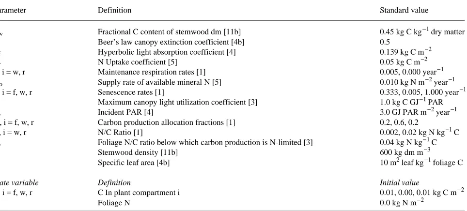
νf is much smaller than this because of two additional loss Table 2. Standard parameter values and initial values of state variables. Parameter values are either based on Comins and McMurtrie (1993) or otherwise represent reasonable estimates. Abbreviations as in Table 1; also f = foliage, w = stemwood, r = fine roots, dm = dry matter. Relevant equation numbers are given in square brackets.
Parameter Definition Standard value
fcw Fractional C content of stemwood dm [11b] 0.45 kg C kg−1 dry matter
k Beer’s law canopy extinction coefficient [4b] 0.5
Kf Hyperbolic light absorption coefficient [4] 0.139 kg C m−2
Kr N Uptake coefficient [5] 0.05 kg C m−2
ri, i = w, r Maintenance respiration rates [1] 0.005, 0.000 year−1
Uo Supply rate of available mineral N [5] 0.010 kg N m−2 year−1
γi, i = f, w, r Senescence rates [1] 0.333, 0.005, 1.000 year−1
εo Maximum canopy light utilization coefficient [3] 1.0 kg C GJ−1 PAR
φo Incident PAR [4] 3.0 GJ PAR m−2 year−1
ηi, i = f, w, r Carbon production allocation fractions [1] 0.2, 0.6, 0.2
νi, i = w, r N/C Ratio [1] 0.002, 0.02 kg N kg−1 C
νo Foliage N/C ratio below which carbon production is N-limited [3] 0.04 kg N kg−1 C
ρ Stemwood density [11b] 600 kg dm m−3
σ Specific leaf area [4b] 10 m2 leaf kg−1 foliage C
State variable Definition Initial value
ci, i = f, w, r C In plant compartment i 0.01, 0.00, 0.01 kg C m−2
terms in the dynamic equation for νf (derived from Equations 1a and 1b), associated with (i) export of nitrogen to stemwood and fine roots, and (ii) the negative effect on νf of dilution by foliage carbon growth. In other words, νf is a ‘‘fast’’ variable relative to cf.
This means that, as cf increases during the canopy-building phase, the value of νf (when measured on the time scale 1/γf)
will lie close to its ‘‘fast-equilibrium’’ value, given by the solution to
dνf
dt = 0 (6a)
at each value of cf. As Figure 2b shows, this is already the case within the first year after planting. Note that the fast-equilib-rium value of νf changes with cf, and is not the same as the long-term equilibrium νf* attained at canopy closure (see Equation B3, Appendix B and Table 3). Equation 6a can be restated as
dnf dt =νf
dcf
dt . (6b)
The advantage of this approximation is that Equation 6b en-ables nf to be eliminated from Equation 1, which therefore reduces to a set of three dynamic equations for cf, cw and cr. Approximation 2: G approaches equilibrium on a single characteristic time scale
In numerical simulations of Equations 1--5, foliage carbon and nitrogen attain their equilibrium values (corresponding to can-opy closure) approximately 7--8 years after planting. This time scale is determined principally by the inverse of the leaf senes-cence rate (e.g., the time to reach 90% canopy closure is approximately 2.3/γf= 6.9 years). Simulations show that the carbon production rate (G) equilibrates on a faster time scale (about 4 years after planting), because G (Equations 2--4) is a saturating function of cf (Figure 2a), and νf is already close to its long-term equilibrium value νf*after about 4 years (Figure 2b, Table 3). The approach of G toward its equilibrium value, G*,can be approximated by the following expression:
G = G∗(1 − e−λt), (7)
Figure 2. Illustration of model approximations. (a) The fraction of incident light absorbed by the canopy (φabs /φo) as a function of foliage carbon (cf), calculated according to Beer’s law (φabs /φo = 1 − exp(−
kσcf), solid line) and a rectangular hyperbolic approximation (Equa-tion 4a, broken line); the two responses have been matched at 50% absorption according to Equation 4b. (b) Changes in foliage N/C ratio (νf = nf /cf) with time since planting, predicted from numerical simu-lations of Equations 1--5 (basic model, solid line) and Equations 1--6 (assuming that νf is a ‘‘fast’’ variable, broken line). (c) Carbon produc-tion (G) as a funcproduc-tion of time since planting (t), predicted from numerical simulations of Equations 1--5 (solid line) and from the analytical approximation given by Equation 7 (broken line). The values for G* and λ in Equation 7 were calculated using the analytical expressions given in Appendices B and C. Parameter values in (a) to (c) are given in Table 2.
Table 3. Stand growth characteristics predicted by the analytical model using parameter values in Table 2. See Table 1 for symbol definitions.
Stand characteristic Equation used Standard value
cf* B6 0.57 kg C m−2
cr* B4 0.19 kg C m−2
cw* 9 56.9 kg C m−2
G* B9 0.95 kg C m−2 year−1
Yg 13b 21.1 m3 ha−1 year−1
nf* nf* = νf*. cf* 9 × 10⁻³ kg N m−2
T 12 18.8 year
U* B10 7.9 × 10⁻³ kg N m−2 year−1
Vw* Vw* = cw*.104/ρfcw 2107 m3 ha−1
Y 13a 17.7 m3 ha−1 year−1
λ C5 0.64 year−1
2.3/λ(1) C5 3.6 year
µw, µr 10, B5 0.01, 1.00 year−1
where λ determines the rate of approach. Equation 7 is increas-ingly accurate the closer G is to equilibrium. The approxima-tion consists of extending this expression back to the initial time of planting (t = 0) when G = 0, implying in effect that the dynamics of G can be characterized by a single time scale (1/λ). As shown in the next section, the advantage of Equa-tion 7 is that it allows the dynamic equaEqua-tion for stemwood carbon (cw, Equation 1c)to be integrated explicitly, giving an analytical expression for cw as a function of stand age (t), which involves the carbon production constants G* and λ.
In Appendix B, G* is derived analytically as a function of the model parameters (see Equation B9). With the aid of Approximation 1 (Equation 6), λ can also be calculated explic-itly in terms of the model parameters (see Equation C5, Appen-dix C). With standard parameter values (Table 2), we find G* = 0.95 kg C m−2 year−1 and λ = 0.64 year−1 (so that G reaches 90% of its equilibrium value at time t = 2.3/λ = 3.6 years after planting). As shown in Figure 2c, Equation 7 gives a reason-able approximation for the variation of carbon production with stand age, although it slightly underestimates G, especially during years 2--4 after planting.
General factors affecting stemwood growth
The constants G* and λ, which characterize the variation of carbon production with stand age according to Equation 7, are calculated as functions of the model parameters in Appendices B and C. Here, however, we examine some general conse-quences of Equation 7 for the relationship of stemwood growth to G* and λ that will be of use in interpreting the response of stemwood growth to changes in nitrogen supply.
Substituting Equation 7 into Equation 1c allows Equation 1c to be integrated explicitly, giving the following expression for stemwood carbon as a function of stand age (t):
cw(t)= cw∗
1 −
λe−µwt−µ
we−λt
λ−µw
, (8)
in which cw* is the equilibrium value of stemwood carbon, given by
cw∗=
ηwG∗
µw
(9)
and where µwis given by
µw=γw+ rw. (10)
Equation 8 describes a sigmoidal growth curve (Figure 3a), with cw increasing from zero toward an asymptotic value, given by Equation 9, that is proportional to carbon production at canopy closure, G*. The shape of the sigmoidal curve is determined by λ and µw; in general λ >> µw because the time scale for carbon production to equilibrate is normally much less than the time scales associated with stemwood mainte-nance respiration and senescence; in the example from Table 3,
λ = 0.64 year−1 and µw= 0.01 year−1.
We now use Equation 8 to calculate the relationship of maximum mean annual stemwood volume increment (Y, m3 ha−1 year−1) and optimal rotation length (T) to the carbon production constants, G* and λ. In carbon terms, the mean annual increment (MAI, kg C m−2 year−1) at time t is defined by cw(t)/t. The optimal rotation length is the time when MAI has a maximum, which coincides with the time when MAI equals the current annual increment (dcw/dt, Equation 1c), as illustrated in Figure 3b (in terms of equivalent volume incre-ments). Therefore, Y (m3 ha−1 year−1) and T satisfy the condi-tions:
ρfcw 104 Y =
cw(T)
T =
dcw
dt(t = T), (11)
where ρ is the stemwood density (kg dry matter m−3), fcw is the stemwood fractional carbon content (kg C kg−1 dry matter), and the factor of 10−4 converts from ha−1 to m−2. Substituting Equation 1c for dcw/dt, and using Equations 7 and 8 to express G and cwas functions of time, the following implicit equation for T can be derived from the second equality in Equation 11:
1 −λe
−µwT−µ
we−λT
λ−µw
= µwT 1 +µwT
(1 − e−λT). (12)
This equation may be solved numerically for T for given values of λ and µw. From Equations 8, 9, 11 and 12, Y is given by:
Y = Yg 1 − e−λT 1 +µwT
, (13a)
where
Yg=ηwG∗ 104
ρfcw
(13b)
is the rate at which carbon production is allocated to stemwood at canopy closure, expressed on a stemwood volume basis (m3 ha−1 year−1), i.e., the gross stemwood volume production at canopy closure. The solution for T from Equation 12 may then be substituted into Equation 13a. With standard parameter values (Table 2), Equations 12 and 13 predict T = 18.8 years and Y = 17.7 m3 ha−1 year−1 (Table 3), which are typical values for fast-growing Eucalyptus species in Australia (West and Mattay 1993).
Although Equations 12 and 13 must be solved numerically, useful analytical approximations to the numerical solutions can be derived by exploiting the fact that λ is typically much greater than µw. As shown in Appendix D, these approxima-tions are given by the following simple expressions:
T ≈
√
2 λµw(14a)
and
Y ≈ Yg 1
1 +
√
2µwλ
, (14b)
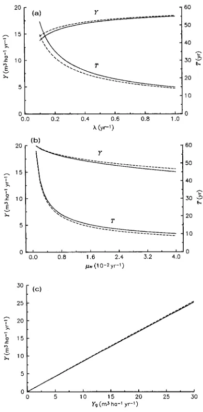
which give T ≈ 17.7 year and Y ≈ 17.9 m3 ha−1 year−1 with standard parameter values (cf. Table 3). These results show explicitly how the optimal rotation length (T) and maximum MAI (Y) can be expected to vary as functions of (i) the time for carbon production to reach equilibrium (∝ 1/λ), (ii) the com-bined rates of stemwood maintenance respiration and senes-cence (µw, Equation 10), and (iii) the gross stemwood volume production rate at canopy closure (Yg, Equation 13b). The value of T depends only on the first two of these factors. As Figure 4 shows, the analytical expressions given by Equation 14 are reasonable approximations to the numerical solutions of Equations 12 and 13.
According to Equation 14a, T increases if carbon production equilibrates more slowly (i.e., if λ decreases), or if the specific rates of stemwood maintenance and senescence decrease (i.e., if µw decreases), as shown in Figures 4a and 4b. Equation 14b implies that Y increases if carbon production equilibrates more
rapidly (i.e., if λ increases), or if stemwood maintenance/se-nescence rates (µw) decrease (Figures 4a and 4b); Y is also directly proportional to Yg (Figure 4c), and hence (see Equa-tion 13b) to carbon producEqua-tion at canopy closure (G*). In quantitative terms, Y and T are relatively insensitive to changes in λ above λ = 1.0 year−1, corresponding to equilibration times for G shorter than about 2 years (Figure 4a). The optimal rotation length is particularly sensitive to changes in µw below about µw = 0.01 year−1, corresponding to specific maintenance and senescence rates of less than 1% per year (Figure 4b).
It is worth noting that Equation 7 also enables analytical
solutions to be found for foliage and fine root carbon as functions of stand age. These solutions have the same form as Equations 8 and 9 for stemwood carbon, with (i) ηw replaced by ηf and ηr, and (ii) µw replaced by γf and µr, respectively.
Dependence of maximum MAI and optimal rotation length on model parameters
According to the above analysis, the sensitivities of Y and T to a given parameter of the model can be interpreted in terms of its influence on each of the three factors λ, µw and Yg. In Appendices B and C, analytical expressions are derived for Yg and λ as functions of the model parameters, and the results of a sensitivity analysis are shown in Table 4.
Maximum MAI (Y)
The parameters to which Y is most sensitive are the stemwood density (ρ), stemwood carbon fraction (fcw) and nitrogen sup-ply rate (Uo). The effect on Y of increases in ρ and fcw is straightforwardly explained in terms of their effect on Yg (Equation 13b).
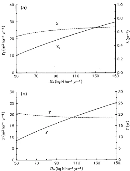
Of major interest to plantation managers is the dependence of Y on Uo. The sensitivity of stemwood growth to changes in Uo is therefore shown more generally in Figure 5. Increasing Uo by 10% leads to a 9% increase in Y, mainly due to its effect on Yg through G*(Table 4, Figure 5a). Over the range of Uo from 50 to 150 kg N ha−1 year−1 there is an approximately linear increase in Y with Uo from 8 to 25 m3 ha−1 year−1, representing an average of 0.17 m3 stemwood volume gained
for each extra kg of nitrogen supplied (Figure 5b).
Maximum MAI is moderately sensitive to the carbon pro-duction parameters (εo, φo, νo), allocation fractions (ηf, ηr) and root N/C ratio (νr).
Optimal rotation length (T)
The optimal rotation length is predicted to be generally much less sensitive than maximum MAI to changes in parameter values (Table 4), including Uo. Over the range of Uo from 50 to 150 kg N ha−1 year−1, T decreases by 14% from 21 to 18 years (Figure 5b), as a result of a 26% increase in λ from 0.53 to 0.67 year−1 (Figures 4a and 5a). The value of T is moderately sensitive to a change in µw (Table 4), the sum of stemwood maintenance respiration and senescence rates, especially at small values of µw (Figure 4b).
Discussion
The relationship between stemwood growth and nitrogen supply
Equations 8 and 9 describe a simple, process-based model of stemwood growth, showing explicitly the main factors in-volved. The variation of stemwood carbon with stand age [cw(t)] is determined by: (i) ηw, the stemwood allocation frac-tion, (ii) G*, the equilibrium value of carbon production (G),
Table 4. Predicted percentage changes (∆) in Yg (Equation 13b), λ (Equation C5), Y (Equation 13a) and T (Equation 12) due to a 10% increase in individual model parameters from the reference case de-scribed by Tables 2 and 3. See Tables 1 and 2 for symbol definitions. Sensitivity to the three allocation parameters was assessed by varying
ηf and ηr with ηw = 1 −ηf−ηr as indicated below. Note that ∆T ≈
−∆λ/2 in accordance with Equation 14a.
Parameter ∆Yg ∆λ ∆Y ∆T
fcw −9.0 0 −9.0 0
Kf −0.7 −0.8 −0.7 +0.4
Kr −1.9 −2.9 −2.1 +1.6
Uo +8.9 +1.4 +9.1 −0.8
γf −0.7 +3.0 −0.4 −1.6
εo +3.3 +2.0 +3.4 −1.0
φo +3.3 +2.0 +3.4 −1.0
ηf(1) −5.5 −1.3 −5.6 +0.7
ηr(2) −5.4 +3.1 −5.1 -1.6
µw 0 0 −0.8 −4.3
µr −1.9 +2.4 −1.7 −1.3
νw −1.3 +0.1 −1.3 0
νr −4.3 +0.3 −4.2 −0.2
νo −3.3 −2.0 −3.5 +1.1
ρ −9.0 0 −9.0 0
1 Allocation fractions {η
f, ηw, ηr}= {0.22, 0.58, 0.20} 2 Allocation fractions {η
f, ηw, ηr}= {0.20, 0.58, 0.22}
Figure 5. The predicted dependence of (a) Yg (gross stemwood volume productivity at canopy closure, solid line), and λ (∝ 1/equilibration time for G, broken line), and (b)Y (solid line) and T (broken line) on
(iii) λ, the rate at which G approaches G*, and (iv) µw, the combined specific rate of stemwood maintenance respiration and senescence. The simple expressions for the optimal rota-tion length (T) and maximum MAI (Y), given by Equarota-tion 14, are of particular relevance for forest management.
The effect of nitrogen supply (Uo) on maximum MAI and optimal rotation length occurs through its effect on the carbon production constants, G* and λ, which we were able to calcu-late as analytical functions of the model parameters. The effect of Uo on maximum MAI (Y) occurs mainly through its effect on G*, the equilibrium carbon production at canopy closure. The results in Figures 4 and 5 show that G* (and therefore Y) responds linearly to Uo. This response is related to our assump-tion that the light utilizaassump-tion coefficient (ε) is proportional to the foliage N/C ratio when nitrogen is limiting (Equation 3a), and the fact that nitrogen remained limiting (i.e., νf < νo) over the range of Uo considered. The effect of Uo on the optimal rotation length (T) occurs only through its effect on λ, the rate at which carbon production equilibrates. It is worth noting from Appendices B and C that G* and λ are not independent, and that an increase in equilibrium carbon production is asso-ciated with a decrease in the time to reach that equilibrium (Figure 5a).
The value of T is much less sensitive than Y to a change in nitrogen supply, Uo (Figure 5b). As noted earlier, this result follows from the prediction that the optimal rotation length responds to nitrogen supply only via changes in the equilibra-tion rate for carbon producequilibra-tion (λ, see Equation 14a), and that
λ is relatively insensitive to Uo (Figure 5a). With reference to Equation 14a, T may be expected to decrease more rapidly with increasing Uo if stemwood maintenance respiration (µw) increases with Uo due to changes in tissue nitrogen concentra-tion (cf. Ryan 1991, 1995). As the model stands, however, the predicted behavior is broadly consistent with general yield tables for Pinus radiata D. Don in South Australia (see Lewis et al. 1976, their Figure V.2) and with some examples of Eucalyptus yield tables from several countries given in FAO (1979, Chapter 11), which show that the effect of changes in site quality on the age of maximum MAI is much smaller than the effect on the value of the maximum MAI itself.
The analytical expressions for Y and T (Equation 14) be-come invalid at very low nitrogen supply rates, when λ be-comes so small that the condition λ >> µw no longer holds. For the parameter values in Table 2, λ = µw when Uo≈ 15 kg N ha−1 year−1, at which point the stemwood growth curve is no longer sigmoidal, and the concepts of maximum MAI and optimal rotation length break down.
Critical assumptions of the model
There are four key simplifying assumptions in our analysis that should be borne in mind when using the model as the basis for specific applications (e.g., Dewar and McMurtrie 1996, fol-lowing article). First, the validity of Equations 8 and 14 de-pends on the assumption that the approach of G toward its equilibrium value can be characterized by a single time scale (1/λ), as expressed by Equation 7. For the model of McMurtrie and Wolf (1983) and McMurtrie (1991) that we started with
(Equations 1--5), this assumption appears reasonable (Figure 2c). If the behavior of G predicted by more complex process-based models can also be characterized this way, then Equa-tions 8 and 14 provide a useful general framework with which to interpret the output of these models.
Second, the present model assumes that the decrease in stemwood volume increment in old stands (Figure 3b) is caused by increasing stemwood maintenance respiration and senescence (described by the parameter µw), with foliage biomass (cf) and carbon production (G, Figure 2c) remaining constant after canopy closure. This interpretation of the ob-served decline in the aboveground productivity of older stands, though widely accepted for many years, has not been rigor-ously tested and has been questioned (Ryan and Waring 1992). Other hypotheses have been proposed (e.g., Murty et al. 1996), including reduced stomatal conductance (thereby reducing ε) and decreased nutrient availability (Uo). It is clearly important to examine the implications of these alternative hypotheses for predictions of stemwood growth, maximum MAI and optimal rotation lengths.
Third, it is assumed that the allocation fractions are fixed constants during stand development. This is clearly not the case in real stands, particularly during the years before canopy closure. Numerous studies of coniferous species have shown that partitioning of aboveground dry matter production to wood tends to increase at the expense of foliage as stands approach canopy closure, but is approximately constant after canopy closure (see reviews by Cannell 1985, Gower et al. 1994). There are few data on changes in allocation between roots and foliage for different-aged stands of the same species. However, fertilization studies and comparisons between trees grown on fertile and nutrient-poor sites (Gower et al. 1994) suggest that allocation to root growth may increase if nutrient availability declines with stand age, for example due to immo-bilization of nutrients by woody litter in old stands (Pearson et al. 1987). There are several approaches to modeling allocation dynamically (Cannell and Dewar 1994). However, it is un-likely that dynamic allocation could be incorporated into the present analytical framework, and its implications for stem-wood growth would probably require numerical simulation. The assumption of constant allocation fractions provides a useful first approximation, but its limitations are acknow-ledged and will be critically examined elsewhere.
Acknowledgments
This work was supported by the UK NERC through its TIGER (Terrestrial Initiative in Global Environmental Research) programme (grant GST/91/15), the Australia-New Zealand-UK Tripartite Agree-ment on Climate Change Research, the NGAC Dedicated Greenhouse Research Grants Scheme and the Australian Research Council.]
References
Cannell, M.G.R. 1985. Dry matter partitioning in tree crops. In Attrib-utes of Trees as Crop Plants. Eds. M.G.R. Cannell and J.E. Jackson. Inst. Terrestrial Ecology, Huntingdon, UK, pp 160--193.
Cannell, M.G.R. and R.C. Dewar. 1994. Carbon allocation in trees: a review of concepts for modelling. Adv. Ecol. Res. 25:59--104. Comins, H.N. and R.E. McMurtrie. 1993. Long-term biotic response
of nutrient-limited forest ecosystems to CO2-enrichment: equilib-rium behaviour of integrated plant-soil models. Ecol. Appl. 3:666--681.
Dewar, R.C. and R.E. McMurtrie. 1996. Sustainable stemwood yield in relation to the nitrogen balance of forest plantations: a model analysis. Tree Physiol. 16:173--182.
Dixon, R.K., R.S. Meldahl, G.A. Ruark and W.G. Warren. 1990. Process modeling of forest growth responses to environmental stress. Timber Press, Portland, Oregon, USA. 441 p.
FAO. 1979. Eucalypts for Planting. FAO Forestry Series No. 11. Food and Agriculture Organization of the United Nations, Rome, 677 p. Gower, S.T., H.L. Gholz, K. Nakane and V.C. Baldwin. 1994. Produc-tion and carbon allocaProduc-tion patterns of pine forests. Ecol. Bull. 43:115--135.
Kirschbaum, M.U.F., D.A. King, H.N. Comins, R.E. McMurtrie, B.E. Medlyn, S. Pongracic, D. Murty, H. Keith, R.J. Raison, P.K. Khanna and D.W. Sheriff. 1994. Modelling forest response to increasing CO2 concentration under nutrient-limited conditions. Plant Cell
Environ. 17:1081--1099.
Lewis, N.B., A. Keeves and J.W. Leech. 1976. Yield regulation in South Australian Pinus radiata plantations. Bull. No. 23. Woods and Forests Dept., SA, Australia.
McMurtrie, R.E. 1985. Forest productivity in relation to carbon parti-tioning and nutrient cycling: a mathematical model. In Attributes of Trees as Crop Plants. Eds. M.G.R. Cannell and J.E. Jackson. Inst. Terrestrial Ecology, Huntingdon, UK, pp 194--207.
McMurtrie, R.E. 1991. Relationship of forest productivity to nutrient and carbon supply----a modeling analysis. Tree Physiol. 9:87--99. McMurtrie, R.E. and L. Wolf. 1983. Above- and below-ground growth
of forest stands: a carbon budget model. Ann. Bot. 52:437--448. Murty, D., R.E. McMurtrie and M.G. Ryan. 1995. Declining forest
productivity in ageing forest stands----a modeling analysis of alter-native hypotheses. Tree Physiol. 16:187--200.
Parton, W.J., D.S. Schimel, C.V. Cole and D.S. Ojima. 1987. Analysis of factors controlling soil organic matter levels in Great Plains grasslands. Soil Sc. Soc. Am. J. 51:1173--1179.
Pearson, J.A., D.H. Knight and T.J. Fahey. 1987. Biomass and nutrient accumulation during stand development in Wyoming lodgepole pine forests. Ecology 68:1966--1973.
Ryan, M.G. 1991. The effects of climate change on plant respiration. Ecol. Appl. 1:157--167.
Ryan, M.G. 1995. Foliar maintenance respiration of subalpine and boreal trees and shrubs in relation to nitrogen content. Plant Cell Environ. 18:765--772.
Ryan, M.G. and R.H. Waring. 1992. Maintenance respiration and stand development in a subalpine lodgepole pine forest. Ecology 73:2100--2108.
Schimel, D.S., W.J. Parton, T.G.F. Kittel, D.S. Ojima and C.V. Cole. 1990. Grassland biogeochemistry: links to atmospheric processes. Clim. Change 17:13--25.
West, P.W. and J.P. Mattay. 1993. Yield prediction models and com-parative growth rates for six Eucalyptus species. Aust. For. 56:211--225.
Appendix A. Nitrogen uptake by trees (U, Equation 5) Let Uo be the rate of nitrogen input to the soil mineral nitrogen pool (Nmin ) due to net mineralization, fertilizer application, atmospheric deposition and fixation. The rate of change of the soil mineral nitrogen pool is therefore:
dNmin
dt = Uo− U − Uv− L,
(A1)
where U is the rate of nitrogen uptake by trees, Uv is the rate of nitrogen uptake by other vegetation and micro-organisms, and L is the external loss of nitrogen from the ecosystem due to leaching and gaseous emission losses. The rate U is assumed to be proportional to the amount of root present (cr) and to Nmin:
U =σcrNmin, (A2)
where σ describes the nitrogen uptake capacity of tree roots. Uv and L are also assumed to be proportional to Nmin : Equation A5 is sufficiently small compared to the time scales on which changes in Uo and cr occur, then Nmin can be taken as a ‘‘fast’’ variable relative to Uo and cr. The uptake rate U can then be approximated by replacing Nmin in Equation A2 with its fast-equilibrium value Nmin*. Substituting Equation A6 into Equation A2 and dividing by σ gives the rate of nitrogen uptake by roots as:
U = Uocr cr+(σv+ ln)/σ
. (A7)
given by
Kr=
σv+ ln
σ (A8)
and so reflects the nitrogen absorption capacity of tree roots, the intensity of competition for nitrogen from other vegetation, and the intrinsic loss rate of nitrogen out of the system.
Appendix B. Derivation of G* (equilibrium carbon pro-duction) as a function of the model parameters
From Equation 1a, G* is related to the amount of foliage at canopy closure, cf*, by
G∗=γfcf∗ ηf
. (B1)
Substituting the expressions for ε(νf) and φabs (cf), given by Equations 3a and 4a, into Equation 2 for G, this relationship can be re-written as:
be calculated by combining Equations 1a and 1b to give:
νf∗=
where U* is the nitrogen uptake rate at canopy closure. From Equation 5, U*depends on the equilibrium root carbon, cr*, which, from Equations 1a and 1d, is simply related to equilib-rium foliage carbon by:
Combining Equation 5 with Equations B2--B4 then leads to a quadratic equation for cf*, the solution to which can be written as:
cf∗= Kfx. (B6)
The dimensionless quantity x is given by:
x =1 +α+β
where the three dimensionless parameter combinations α, β and δ are given by:
Finally, Equation B6 may be substituted into Equation B1 to give
G∗=Kfγf ηf
x. (B9)
Equation B9 may be inserted into Equation 15b to obtain Yg. The corresponding expression for U* can be obtained by combining Equations 5, B4 and B6, to give:
U∗= Uox
x +β . (B10)
Appendix C. Derivation of λ (rate of equilibration of carbon production) as a function of the model parameters Equations 1a, 1b and 1d governing the dynamics of cf, nf and cr may be replaced by an equivalent system of equations for G, nf and U using the relationships given by Equations 2, 3a, 4a and 5. Using approximation 1 (foliage N/C is a ‘‘fast’’ variable) to eliminate nf, this system can be reduced to the following two coupled dynamic equations for G and U alone:
dG
B). Mathematically, the parameter λ in Equation 7 is then equal to −λ1, where λ1 is the least negative eigenvalue of the dynam-ics of the linearized G--U system.
Standard eigenvalue analysis gives:
λ1=
−µr− A +√(µr− A)2+ 4B
2 (C3a)
and
λ2=
−µr− A −√(µr− A)2+ 4B
2 (C3b)
in which
A =γf(2x +α+ 1)(x +β)
δ−α(x +β) (C4a)
and
B = γfµrβδ
(x +β)(δ−α(x +β)) , (C4b)
where x, α, β and δ are given in Appendix B (Equations B7--B8). The least negative eigenvalue is λ1 (Equation C3a), and so, setting λ = −λ1, we have:
λ=µr+ A −√(µr− A)2+ 4B
2 . (C5)
With the standard parameter values in Table 2, we find λ1=
−0.640 and λ2 = −1.512. Although λ2 only differs from λ1 by a factor of 2.3, the use of the single exponential term exp(−λt) in Equation 7 appears to be justified by the close agreement between the calculated stemwood growth curve based on Equation 7 (i.e., Equation 8) and that based on the full numeri-cal simulation of Equations 1--5, as shown in Figure 3.
Appendix D. Derivation of analytical expressions for T and Y (Equation 14)
The implicit equation for T (Equation 12) may be simplified
by exploiting the fact that λ is typically much greater than µw. Substituting the values of λ, µw and T from Table 3 into the left-hand side of Equation 12, the term µwexp(−λT) ≈ 6 × 10⁻⁸ year−1 is negligible compared to the term λexp(−µwT) ≈ 0.5 year−1. In addition, on the right-hand side of Equation 12, the term exp(−λT) ≈ 6 × 10⁻⁶ is negligible compared to 1. There-fore, Equation 12 may be approximated by:
1 −λe
−µwT λ−µw
= µwT 1 +µwT
. (D1)
Noting that µwT ≈ 0.19, this equation can be simplified further by expanding each side as a power series up to second order in
µwT, to give:
1 − λ
λ−µw
1 −µwT + (µwT)2
2
=µwT −(µwT)
2. (D2)
This is a quadratic equation for µwT, which may be solved to give the solution for T as:
T = 1 λ− 2µw
√
2λ
µw
− 3 − 1
. (D3)
Because λ >> µw, we have λ− 2µw≈λ and the expression in square brackets may be approximated by √2λ/µw, giving the
approximation:
T ≈
√
2 λµw. (D4)
Substituting this result into the equation for Y (Equation 13a) (in which the term exp(−λT) can similarly be neglected) then gives:
Y ≈ Yg
1 +
√
2µwλ