Biostatistics 102:
Quantitative Data – Parametric
& Non-parametric Tests
Y H Chan
Clinical Trials and Epidemiology Research Unit 226 Outram Road Blk A #02-02 Singapore 169039
Y H Chan, PhD Head of Biostatistics
Correspondence to:
Y H Chan Tel: (65) 6317 2121 Fax: (65) 6317 2122 Email: chanyh@ cteru.com.sg
In this article, we are going to discuss on the statistical tests available to analyse continuous outcome variables. The parametric tests will be applied when normality (and homogeneity of variance) assumptions are satisfied otherwise the equivalent non-parametric test will be used (see table I).
TableI. Parametric vs Non-Parametric tests.
Parametric Non-Parametric
1 Sample T-test Sign Test/Wilcoxon Signed Rank test
Paired T-test Sign Test/Wilcoxon Signed Rank test
2 Sample T-test Mann Whitney U test/Wilcoxon Sum Rank test
ANOVA Kruskal Wallis test
We shall look at various examples to understand when each test is being used.
1 SAMPLE T-TEST
The 1-Sample T test procedure determines whether the mean of a single variable differs from a specified constant. For example, we are interested to find out whether subjects with acute chest pain have abnormal systolic (normal = 120 mmHg) and/or diastolic (normal = 80 mmHg) blood pressures. 500 subjects presenting themselves to an emergency physician were enrolled.
Assumption for 1 sample T test: Data are normally distributed. We have discussed in the last article(1) on how to check
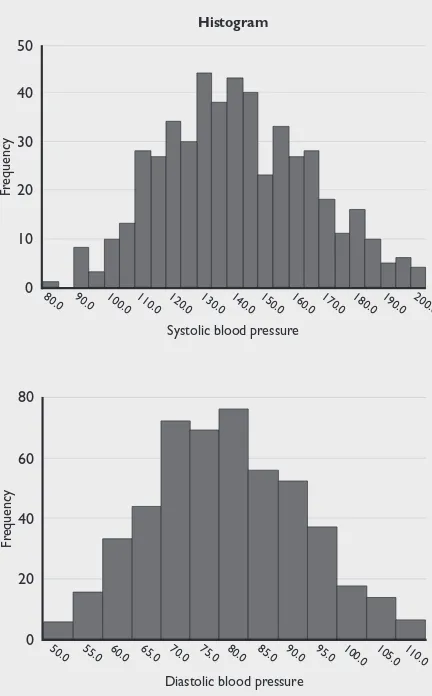
the normality assumption of a quantitative data. One issue being highlighted was that these formal normality tests are very sensitive to the sample size of the variable concerned. As seen here, table II shows that the normality assumptions for both the systolic and diastolic blood pressures are violated but basing on their histograms (see figure 1), normality assumptions are feasible.
Table II. Formal normality tests.
Tests of Normality
Kolmogorov-Smirnova Shapiro-Wilk
Statistic df Sig. Statistic df Sig.
systolic blood pressure .049 500 .006 .990 500 .002
diastolic blood pressure .042 500 .032 .992 500 .011
a Lilliefors Significance Correction.
Figure 1. Histograms of Systolic & Diastolic blood pressures.
0
Systolic blood pressure 20
30 40 50
10
Fr
equency
Histogram
80.0 90.0 100.0 110.0 120.0 130.0 140.0 150.0 160.0 170.0 180.0 190.0 200.0
0
Diastolic blood pressure 40
60 80
20
Fr
equency
50.0 55.0 60.0 65.0 70.0 75.0 80.0 85.0 90.0 95.0 100.0 105.0 110.0
So with the normality assumptions satisfied, we could use the 1 Sample T-test to check whether the systolic and diastolic blood pressures for these subjects are statistically different from the norms of 120 mmHg and 80 mmHg respectively.
Firstly, a simple descriptive would give us some idea, see table III.
Table III. Descriptive statistics for the systolic & diastolic BP.
Mean Std Minimum Maximum Median Deviation
systolic
blood pressure 140.51 24.08 79.00 200.00 139.00
diastolic
In the Sign test, the magnitude of the differences between the variable and the norm is not taken into consideration when deriving the significance. It uses the number of positives and negatives of the differences. Thus if there were nearly equal numbers of positives and negatives, then no statistical significance will be found regardless of the magnitude of the positives/negatives. The Wilcoxon Signed Rank test, on the other hand, uses the magnitude of the positives/negatives as ranks in the calculation of the significance, thus a more sensitive test.
PAIRED T-TEST
When the interest is in the before and after responses of an outcome (within group comparison), say, the systolic BP before and after an intervention, the paired T-test would be applied.
Table VIII shows the descriptive statistics for the before and after intervention systolic BPs of 167 subjects.
To perform a 1 Sample T-test, in SPSS, use
Analyze, Compare Means, One-Sample T test. For systolic, put test value = 120 and for diastolic put test value = 80 (we have to do each test separately). Tables IV & V shows the SPSS output.
Table IV. 1 Sample T-test for systolic BP testing at 120 mmHg.
One-Sample Test
Test Value = 120
95% Confidence Interval of the
Difference
t df Sig. Mean Lower Upper (2-tailed) Difference
systolic blood
pressure 19.046 499 .000 20.5080 18.3925 22.6235
Table V. 1 Sample T-test for diastolic BP testing at 80 mmHg.
One-Sample Test
Test Value = 80
95% Confidence Interval of the
Difference
t df Sig. Mean Lower Upper (2-tailed) Difference
diastolic blood
pressure -2.345 499 .019 -1.3540 -2.4886 -0.2194
These subjects had a much higher systolic BP (p<0.001, difference = 20.5, 95% CI 18.4 to 22.6) compared to the norm of 120 mmHg. This difference is clinically ‘relevant’ too. For the diastolic BP, though there was a statistical significance of 1.35 (95% CI 0.22 to 2.5, p = 0.019) lower than the norm of 80 mmHg, this difference may not be of clinical significance. By now, we should realize that the p-value is significantly affected by sample size(2), thus
we should be looking at the clinical significance first then the statistical significance.
If the normality assumptions were not satisfied, then the equivalent non-parametric Sign test or Wilcoxon Signed Rank test would be used. In SPSS, before we could perform the non-parametric analysis, we will have to create a new variable in the dataset, say, sysnorm (which is just a column of 120). Use the Transform, Compute command to do this (likewise, we have to create a new variable, say,
dianorm which is just a column of 80). Then go to
Analyze, Non Parametric tests, 2 related samples
to do the tests (we can do both tests for systolic and diastolic simultaneously, Tables VI & VII show the SPSS outputs). In this case, we are analyzing the medians of the variables rather than their means.
Table VIII. Descriptive statistics for the before & after intervention systolic BP.
Std
Mean Deviation Minimum Maximum Median
systolic
BP before 142.31 22.38 90.00 200.00 139.00
systolic
BP after 137.14 24.87 90.00 199.00 137.00 Table VI. Wilcoxon Signed Rank tests.
Test Statisticsc
SYSTOLIC - DIASTOLI -systolic blood diastolic blood pressure pressure
z -14.965 -2.474
Asymp. Sig. (2-tailed) .000 .013
c Wilcoxon Signed Ranks test.
Table VII. Sign test.
Test Statisticsa
SYSTOLIC - DIASTOLI -systolic blood diastolic blood pressure pressure
z -13.169 -2.343
Asymp. Sig. (2-tailed) .000 .019
a Sign Test.
Assumption for the Paired T test:
The difference between the before & after is normally distributed
2. Homogeneity of variance (The population variances are equal).
3. The 2 groups are independent random samples.
The 3rd assumption is easily checked from the
design of the experiment – each subject can only be in one of the groups or intervention. The 1st assumption
of normality is also easily checked by using the
Explore option in SPSS (with group declared in the Factor list – this will produce normality checks for each group separately). Normality assumptions must be satisfied for both groups for the 2 Sample T test to be applied. Lastly, the 2nd assumption of homogeneity
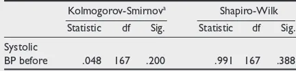
of variance will be given in the 2 Sample T test analysis. assumption and figure 2 shows the corresponding
histogram.
Table IX. Normality assumption checks.
Kolmogorov-Smirnova Shapiro-Wilk
Statistic df Sig. Statistic df Sig.
Systolic
BP before .048 167 .200 .991 167 .388
Table X. Paired T-test for the Before & After intervention systolic BP.
Paired Differences
95% Confidence Interval of the
Difference
Std.
Std. Error Sig. (2-Mean Deviation (2-Mean Lower Upper t df tailed)
Pair 1
systolic BP before
5.17 34.11 2.64 -.04 10.38 1.958 166 .052 systolic BP after
Table XII. Wilcoxon Signed Rank test on the difference on the Before & After intervention systolic BP.
Test Statisticsb
systolic BP after -systolic BP before
z -1.803a
Asymp. Sig. (2-tailed) .071
a Based on positive ranks b Wilcoxon Signed Ranks Test
Table XIII. Descriptive statistics of Systolic BP by group.
Mean Std Minimum Maximum Median Deviation
over-weight 141.65 23.06 90.00 200.00 138.00
normal-weight 97.12 10.82 80.00 132.00 100.00 0
systolic BP before - after 20
30
10
Fr
equency
-70.0 -60.0 -50.0 -40.0 -30.0 -20.0 -10.0 0.0 10.0 20.030.040.0 50.060.0 70.0 80.0 90.0 100.0
Figure 2. Histogram of the difference between the Before & After intervention systolic BP.
Since the normality assumption is satisfied, we can use the paired T-test to perform the analysis: In SPSS, use Analyze, Compare Means, Paired Samples T test. Table X shows the SPSS output for the paired T-test.
Clinically there was a mean reduction of 5.17 mmHg but this was not statistically significant (p = 0.052). Should we then increase the sample size to ‘chase after the p-value’? We shall discuss this issue at the end of this article.
Alternatively, we can use the 1-Sampe T test (with test value = 0) on the difference between the Before & After to check whether there was a statistical significance; see Table XI.
In the event that the normality assumption was not satisfied, we will use the Wicoxon Signed Rank test to perform the comparison on the medians. In SPSS, use Analyze, Non Parametric tests, 2 related samples: table XII shows the SPSS output.
2 SAMPLE T-TEST
When our interest is the Between-Group comparison, the 2 Sample T test would be applied. For example, we want to compare the systolic BP between the normal weight and the over-weight (a proper power analysis should be done before embarking on the study(2)). 250 subjects for each group were recruited.
Table XIII gives the descriptive statistics.
Assumptions of the 2 Sample T test:
1. Observations are normally distributed in each population.
Table XI. 1 Sample T test for the difference between the Before & After intervention systolic BP.
One-Sample Test
Test Value = 0
95% Confidence Interval of the Difference
t df Sig. Mean Lower Upper (2-tailed) Difference
systolic BP
To perform a 2 Sample T test, in SPSS, use
Analyze, Compare Means, Independent Samples T-test. Table XIV shows the SPSS output.
The Levene’s Test for equality of variances checks the 2nd assumption. The Null hypothesis is:
Equal Variances assumed. The Sig value (given in the 3rd column) shows that the Null hypothesis of
equal variances was rejected and SPSS adjusts the results for us. In this case we have to read off the p-value (Sig 2-tailed) from the 2nd line (equal variances
not assumed) rather than from the 1st line (equal
variances assumed). As expected, there was a significant difference in the systolic BP between the over-weight and normal (p<0.001, difference = 44.53, 95% CI 41.36 to 47.69 mmHg)
When normality assumptions are not satisfied for any one or both of the groups, the equivalent non-parametric Mann Whitney U/Wilcoxon Ranked Sum tests should be applied. In SPSS, use Analyze, Non Parametric tests, 2 Independent Samples. Table XV shows the results for the non-parametric test.
Table XV. Mann Whitney U & Wilcoxon Rank Sum tests.
Test Statisticsa
BPSYS
Mann-Whitney U 1664.000
Wilcoxon W 33039.000
z -18.454
Asymp. Sig. (2-tailed) .000
a Grouping Variable: TRT.
Observe that only 1 p-value will be given for both Mann Whitney U and Wilcoxon Rank Sum tests.
ANOVA (ANALYSIS OF ONE WAY VARIANCE)
The ANOVA is just an extension of the 2-Sample T test – when there are more than 2 groups to be compared. The 3 assumptions for the 2-Sample T test also apply for the ANOVA. Let’s say, this time we have 3 weight groups (normal, under and over weight), the descriptive statistics is given in Table XVI.
After checking for the normality assumptions, to perform an ANOVA, in SPSS, use Analyze, Compare Means, One-Way ANOVA. Click on Options and tick the Homogeneity of Variance test. Tables XVII & XVIII shows the results for the homogeneity of variance and ANOVA tests respectively.
Table XVII. Homogeneity of Variance test.
Test of Homogeneity of variances
systolic BP
Levene statistic df1 df2 Sig.
4.249 2 296 .090
The Null hypothesis is: Equal Variances assumed. Since p = 0.09>0.05, we cannot reject the null hypothesis of equal variance.
Table XVIII. ANOVA results.
ANOVA
systolic BP
Sum of df Mean F Sig.
Squares Square
Between Groups 72943.542 2 36471.771 61.126 .000
Within Groups 176613.970 296 596.669
Total 249557.512 298
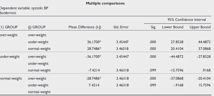
The Null Hypothesis: All the groups’ means are equal. Since p<0.001, not all the groups’ means are equal. We would want to carry out a post-hoc test to determine where the differences were. In SPSS, under the ANOVA, click on the Post Hoc button and tick Bonferroni(3) (this method is most commonly
used and rather conservative in testing for multiple Table XIV. 2 Sample T test.
Independent Samples Test
Levene’s Test for
Equality of Variances t-test for Equality of Means
95% Confidence F Sig. t df Sig. Mean Std. Error Interval of the
(2-tailed) Difference Difference Difference
Lower Upper
Equal variances assumed 131.183 .000 27.638 498 .000 44.5280 1.61111 41.36258 47.69342
Equal variances not assumed 27.638 353.465 .000 44.5280 1.61111 41.35943 47.69657
Table XVI. Descriptive statistics of Systolic BP by weight groups.
Mean Std Minimum Maximum Median
Deviation
over-weight 140.89 24.65 90.00 195.00 137.50
under-weight 104.72 21.58 80.00 186.00 100.00
comparisons). Table XIX shows the post-hoc multiple comparisons using Bonferroni adjustments.
The systolic BP of the over-weights were statistically (and clinically) higher than the other 2 weight groups but there was no statistical difference between the normal and under weights (p = 0.099). If we have carried out multiple 2 Sample T tests on our own, we have to adjust the type 1 error manually. By Bonferroni, we have to multiply the p-value obtained by the number of comparisons performed. For 3 groups, there will be 3 comparisons (ie. A vs B, B vs C & A vs C).
Table XX shows the 2 Sample T-test between the normal and under weights. It seems that there’s also a statistical difference between the 2 groups in systolic BP but taking into account multiple comparison and adjusting for type 1 error, we will have to multiply the p-value (= 0.033) by 3 which gives the same result as in ANOVA post-hoc.
Table XX. 2 Sample T test for Normal vs Under weight.
Independent Samples Test
Levene’s Test for t-test for Equality Equality of Variances of Means
Sig. (2-F Sig. t df tailed)
systolic BP Equal variances
assumed 7.470 .007 -2.153 197 .033
Equal variances
not assumed -2.151 187.71 .033
When normality and homogeneity of variance assumptions are not satisfied, the equivalent non-parametric Kruskal Wallis test will be applied. In SPSS,
use Analyze, Non Parametric tests, k Independent Samples. Table XXI shows the SPSS results.
Table XXI. Kruskal Wallis test on systolic BP for the 3 groups.
Test Statisticsa,b
systolic BP
Chi-Square 101.083
df 2
Asymp. Sig. .000
a Kruskal Wallis Test
b Grouping Variable: GROUP
There was a statistical significant difference amongst the groups. In Kruskal Wallis, there’s no post-hoc option available, we will have to do adjust for the type 1 error manually for multiple comparisons.
TYPE 1 ERROR ADJUSTMENTS
A type 1 error is committed when we reject the Null Hypothesis of no difference is true. If we take the conventional level of statistical significance at 5%, it means that there is a 0.05 (5%) probability that a result as extreme as the critical value could occur just by chance, i.e. the probability of a false positive is 0.05.
There are a few scenarios when adjustments for type 1 error is required:
Multiple comparisons
When we are comparing between 2 treatments A & B with a 5% significance level, the chance of a true negative in this test is 0.95. But when we perform A vs B and A vs C (in a three treatment study), then the probability that neither test will give a significant result when there is no real difference is 0.95 x 0.95 = 0.90; which means the type 1 error has increased to 10%.
Table XIX. ANOVA Bonferroni adjustment for multiple comparisons.
Multiple comparisons Dependent variable: systolic BP
Bonferroni
95% Confidence Interval
(1) GROUP (J) GROUP Mean Difference (I-J) Std. Error Sig. Lower Bound Upper Bound
over-weight over-weight
under-weight 36.1700* 3.45447 .000 27.8528 44.4872
normal-weight 28.7486* 3.46318 .000 20.4104 37.0868
under-weight over-weight -36.1700* 3.45447 .000 -44.4872 -27.8528
under-weight
normal-weight -7.4214 3.46318 .099 -15.7596 .9168
normal-weight over-weight -28.7486* 3.46318 .000 -37.0868 -20.4104
under-weight 7.4214 3.46318 .099 -.9168 15.7596
normal-weight
Table XXII shows the probability of getting a false positive when repeated comparisons at a 5% level of significance are performed. Thus for 3 pairwise comparisons for a 3-treatment groups study (generally, number of pairwise comparisons for a n-group study is given by n(n-1)/2), without performing a type 1 error adjustment, the probability of a false positive is 14%.
Perhaps this p-value will be significant if we increase the sample size. If the sample size was indeed increased, then the obtained p-value will have to be multiplied by 2! The reason being that we are already ‘biased’ by the ‘positive’ trend of the findings and the type 1 error needed to be controlled.
Interim analysis
Normally in large sample size clinical trials, interim analyses are carried out at certain time points to assess the efficacy of the active treatment over the control. This is carried out usually on the ethical basis that perhaps the active treatment is really superior by a larger effect difference than expected (thus a smaller sample size would be sufficient to detect a statistical significance) and we do not want to put further subjects on the control arm. These planned interim analyses with documentations of how the type 1 error adjustments for multiple comparisons must be specifically write-up in the protocol.
CONCLUSIONS
The concentration of the above discussions have been on the application of the relevant tests for different types of designs. The theoretical aspects of the various statistical techniques could be easily referenced from any statistical book.
The next article (Biostatistics 103: Qualitative Data – Test of Independence), we will discuss on the techniques available to analyse categorical variables.
REFERENCES
1. Chan YH. Biostatistics 101: Data presentation, Singapore Medical Journal 2003; Vol 44(6):280-5.
2. Chan YH. Randomised Controlled Trials (RCTs) — sample size: the magic number? Singapore Medical Journal 2003; Vol 44(4):172-4. 3. Bland, JM & DG. Altman. Multiple significance tests: the Bonferroni
method, 1995 British Medical Journal 310:170.
4. Miller RG Jr. Simultaneous Statistical Inference, 2nd ed, 1981, New York, Springer-Verlag.
Table XXII.
Number of
comparisons 1 2 3 4 5 6 7 8 9 10
Probability of
false positive 5% 10% 14% 19% 23% 27% 30% 34% 37% 40%
As mentioned in ANOVA, Bonferroni adjustments (multiplying the p-value obtained in each multiple testing by the number of comparisons) would be the ‘most convenient’ and conservative test. But this test has low power (the ability to detect an existing significant difference) when the number of comparisons is ‘large’. For example with 4 treatment groups, we will have 6 comparisons which means that for every pair-wise p-value obtained, we have to multiply by 6. In such a situation, other multiple comparison techniques like Tukey or Scheffe would be appropriate. Miller (1981)(4) gave a comprehensive review of the
pros and cons of the various methods available for multiple comparisons. In ANOVA, this multiple comparison is automatically handled by the post-hoc option but for Kruskal Wallis test, manual adjustments needed to be carried out by the user which means that the Bonferroni method would normally be used because of it’s simplicity.
‘Chasing’ after the p-value