A Prediction System of Dengue Fever Using Monte Carlo
Method
Mochammad Choirur Roziqin, Achmad Basuki, Tri Harsono
Graduate School of Informatics and Computer Engineering Politeknik Elektronika Negeri Surabaya
Jl. Raya ITS Sukolilo Surabaya 60111, Indonesia Telp: 6231 5947280 Fax : 6231 5946114
E-mail: [email protected], {basuki, trison}@pens.ac.id
Abstract
Dengue fever is an acute disease that clinically can cause death because there is no prediction system to estimate dengue fever cases so it resulted in the growing of dengue fever cases every year. Original data gathering in Jember area that uses technique of partial data gathering has caused data missing. To make this secondary data can be processed in prediction stage there is need to conduct missing imputation by using Monte Carlo method with four different randomization method, followed by data normality test with chi-square, then continued to regression stage. We use MSE (Mean Square Error) to measure prediction error. The smallest MSE result of regression is the best regression model for prediction.
Keywords: Prediction, dengue fever, regression, Jember, Monte Carlo.
1. INTRODUCTION
To obtain valid datas on data proccessing, there is a need to conduct complete and proper data collecting. But oftenly in actual practice of data gathering proccess, the collected information tend to not as complete as the expected. Valid data selection is very important for all kind of used data processing. Valid data is data which is complete, correct, and also consistent. [2] According to Jiawei Han [3] there are several means to be used if there is blank value in data, first is to overlook row with blank value, this method is so ineffective, espescially if the percentage of blank values are high enough that can cause many datas unused. Second means is by filling blank value manually, usually this method is time consuming and unfit to be used in big data collection with many blank values. Third means is by using permanent global value to fill blank value, such as filled them with “unknown”, using average value from attribute that has blank value in it, using average value for all sample according to same class or category and using the most possible value to be filled in in the blank value.
Valid data selection is very important for all kind of used data proccessing and valid data make data processing becomes accurate. After conducting missing imputation on a data, the next step is to predict by using Monte Carlo method. Forecasting is a condition estimation proccess on the future by using data in the past. Forecasting is an activity to dicover value of dependent variable in the future by studying independent variable in the past. Quantitative forecasting method consist of consideration method, regerssion, trend method, input method, output method, and econometric method. [4].
According to Achmad Basuki [5], Monte Carlo method is a method which is the solution is found randomly and repeatedly untill result in expected solution or at least closer to the expected. This method looks very simple because only need a mean of stated solution, then randomize the value untill the expected value is obtained from existing solution model. Actually there are several method that is commonly used in forecasting cases such as Maximum Likelihood Estimator, Naïve Bayessian, or in a case of random data we can use heuristic method to optimize predicted data. But those methods can’t be implemented in this research because there are differences in the data which is in use. In Maximum Likelihood Estimator method, in used data is stationary [6], while in Naïve Bayessian method, the in used data is categorical [7]. In Heuristic method for optimizing forecasting data, the data type must not be a discrit [8]. In this research the in used data is not categorical, but the diskrit one so it is more appropriate to use Monte Carlo method. Because this method able to estimate existing system performance with several condition without deleting blank datas.
performed on the data by using Monte Carlo method. Monte Carlo method is being used in this research because other forecasting system, according to previous research that is stated in related works below, use data that must have complete parameter without data missing. There are many methods to forecast data stationary, one of them is ARIMA method, this method good for stationary data type, but in using ARIMA method we also require the data to be complete without any data missing.
Purpose of this research is to choose the best regression model to forecast dengue fever in the future based on case data of dengue fever and climate data in 2009-2011 in Jember Regency. Data of 2009-2012 is combined and is used to find regression function, and data of 2012 is used as validation data, for measurement of forecasting acuracy will be shown by the value of MSE (Mean Square Error) on each regression.
2. RELATED WORKS
H. Abdul Rahim, et al [9] This paper describes the development of nonlinear autoregressive moving average with exogenous input (NARMAX) models in diagnosing dengue infection. The developed system bases its prediction solely on the bioelectrical impedance parameters and physiological data. Three different NARMAX model order selection criteria namely FPE, AIC and Lipschitz have been evaluated and analyzed. This model is divided two approaches which are unregularized approach and regularized approach. The results show that using Lipschitz number with regularized approach yield better accuracy by 88.40% to diagnose the dengue infections disease. Furthermore, this analysis show that the NARMAX model yield better accuracy as compared to autoregressive moving average with exogenous input (ARMAX) model in diagnosis intelligent system based on the input variables namely gender, weight, vomiting, reactance and the day of the fever as recommended by the outcomes of statistical tests with 76.70% accuracy. This research talk about forecasting of patient infected with dengue fever or not infected with dengue fever by comparing two statistic methods, ARMAX and NARMAX.
experiments is based on the condition of weather data and Dengue Haemorrhagic Fever cases from January 1999 until December 2007 were conducted. Our prediction achieves 85.92% accuracy compared to the actual data.
Dia Bitari Mei Yuana, et al [11] This research develop Fuzy method to predict dengue fever dispersion by using rainfall paramater, the amount of rain days, larva free number, and house index. From the test result of dengue fever dispersion potential method in Jember Regency by using Fuzzy method, we obtained dengue fever dispersion potential that is classified as high with total cases above 30 cases/month that happened in January until March and October until December. Meanwhile in April through September, potency of dengue fever dispersion was classified as low with total cases below 15 cases/month. In high dengue fever potency, value of ABJ tend to be below 95% and HI above 5%. In this research there is incomplete data or blank so there was a must for deleting those datas from data rows in order to show new dataset without performing missing imputation.
Imam Taufik, et al [12] This paper use Monte Carlo simulation to make interpertation of disease speed in community easier. The big amount of dengue fever cases in every year make it possible for every stakeholder become confused on attempt to reduce dengue fever high dispersion rate. This happened because there is no information yet about the amount of dengue fever patients in certain area and the happening of epidemic or Kejadian Luar Biasa (KLB). With Monte Carlo simulation, existence of dengue fever case per individual will be calculated and be conducted an interpretation of disease speed by using computer. This method will make interpretation easier and faster compared to other matematical method. This research only involve one variable, that is a case without looking at climate factor that become one of many factors in dengue fever.
3. ORIGINALITY
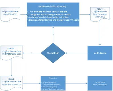
4. SYSTEM DESIGN
Original Parameter Data 2009-2011
Data Randomization with 4 way :
1. Minimum and maximum values in the data 2. Average and around average values in the data 3. Alpha and standart deviasi values in the data
4.Skewness, standart deviasi and averagevalues in the data
Result :
Figure 2. Example of Original Data Parameter
Basing on influencing factors, this research is using four paramater, those are rainfall or curah hujan (CH), the amount of rain days or jumlah hari hujan (HH), larva free number (ABJ), house index (HI) and we will do missing imputation for the next cases by generating random number.
4.2 Randomization Data
In this research we found a lot of blank data on original data paramater. In order to fill those blank datas, we conduct missng imputation by using Monte Carlo method. This steps is done by sorting data in every district in month and year. From those sorted data then we will find value of mean, deviaton standart, and skewness value on each data. Next step is stage of randomization of random number by using Monte Carlo that use four different randomization in 100 times iteration, those are:
1. Randomization of parameter data by minimum limit on data and maximum limit on data.
2. Randomzation of paramater data between average and surrounding average of data.
3. Randomization between deviation standard value and alpha value (95%)
4. Randomization of paramater data between value of average, deviation standard, and skewness.
4.3 Chi-Square Test
In case of testing those datas which are resulted from randomization procces, data is classified as good if the data has normal distribution. Because the amount of data in Jember is 31 district then we use Chi Square Test for data normality test [13].
= Expected frequencies
After calculating exponential chi value, then those values is compared to exponential chi table with alpha of 5% and dk= k-1. If Xh2 < Xt2then we can
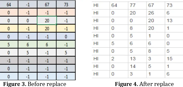
conclude that the data is originated from population with normal distribution. To make calculation of exponential chi easier, then the score of research data is arranged in table of frequencies distribution. After knowing data distribution from those generation of random number with four randomization then data with normal distribution is used to fill in data blankness in original data paramater.
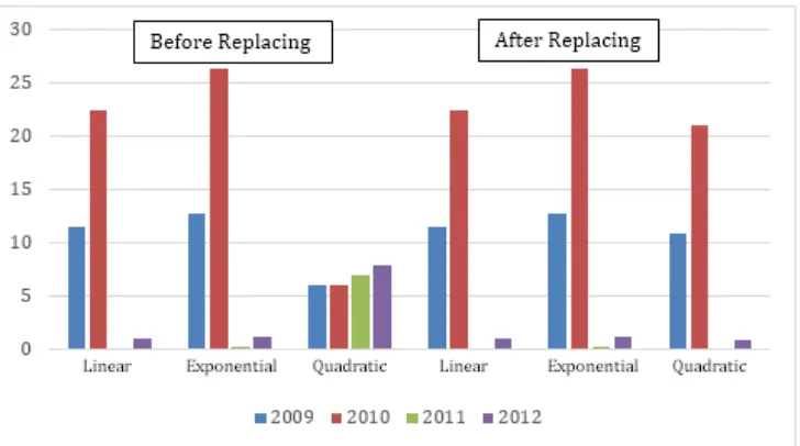
Figure 3. Before replace Figure 4. After replace
4.4 Regression
Regression analysis has characteristic of asymetry or two ways. Regression technique makes a prediction by a value from one variable (independent variable) to another variable (dependent variable). In this case, the purpose is not intended to make perfect prediction. But with information on independent variable, we try to make error in independent variable prediction as low as possible.
In regression, variable we are predicting is called as criterium and variable that is used for predicting is called as predictor. Equation that shows relation between criterium variable and predictor variable is called as regression equation. In this research, we use analysis of four regression, those are:
a) Linear
Linear regression equation is as follow:
Yt = predicted score a = Y intercept
Value of a dan b is obtained from formula:
b) Exponential
Exponential regression equation is as follow:
Yt = predicted score a = Y intercept
b = the slope of the line t = time period
But in doing the calculation, the equation above can be changed to semi log form, that make a process of finding a value and b value easier.
c) Quadratic
Quadratic regression equation is as follow:
Yt = predicted score a = Y intercept
b = the slope of the line t = time period
d) Monte Carlo Linear
Monte Carlo linear is regression method that we try to develop. This method is a development from simple linear regression. Equation of this method is similar to equation of linear regression, that is:
Yt = predicted score a = Y intercept
b = the slope of the line t = time period
The difference is Y value and t value in Monte Carlo linear regression is filled with value of Y and t as results of linear regression which is followed by randomization process with 1000 times iteration to obtain the best result.
e) MSE (Mean Square Error)
Mean Square Error according to Pakaja (2012), Mean Square Error (MSE) is another method to evaluate forecasting method. Each error or residu is being exponentiated. This method set a rule for big forecasting error because those errors is being exponentiated. MSE is a second mean to measure overall forecasting error. MSE itself is average value of the difference in exponential value between forecasted value and observed value. The minus of MSE usage is MSE tend to show big deviation because of the exponentialization. After regression proccess is performed, then MSE of data is calculated with formula as follow:
After calculating MSE on each regression then MSE among regression is compared. Variable in prediction (Y) in this research is total cases and predictor variable (x) is rainfall, rain days, larva free number, and house index.
5.EXPERIMENT AND ANALYSIS
Experiment anad analysis consist of 5.1 Missing Imputation, 5.2 Regression Experiment and the last 5.3 Prediction.
5.1 Missing Imputation
Because data in this research is too much and big then we only give ilustration like explanation below.
Table 1. Table of original data paramater example
CH 110 90 200 150 75 0 56 170 250
Kasus (Y) -1 8 5 3 0 5 9 4 0
Table 1 above shows data in our research that contain missing imputation. In previous research that is stated in related works, if data missing is present then we have to delete 1 rule. So, cases (Y) above is deleted and not in use anymore. The difference between our research and previous one is if by chance there is blank data then we will fill those blank data using Monte Carlo method with four different randomization method.
1. Paramater of original data randomization with minimum limit on data anda maximum limit on data.
Table 2. Table of original data parameter after being treated with first randomization method
CH 110 90 200 150 75 0 56 170 250
Kasus (Y) -1 8 5 3 0 5 9 4 0
First randomization means randomize between minimum value and maximum value on data, in cases date (Y) above we randomize between 0 value until 9 as much as 100 iteration. There is no rule to determine the amount of iteration. After being randomized by 100 times iteration then it will show random value such in the table below.
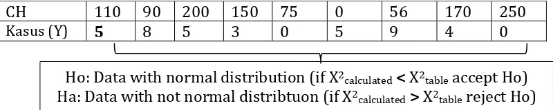
Table 3. Test of data by using chi-square test
CH 110 90 200 150 75 0 56 170 250
Kasus (Y) 5 8 5 3 0 5 9 4 0
Table of data above shows the data which is blank in the beginning (-1) then have been filled with data of random number generation, in this case is 5. After that, to check the normality of generated data, we do chi square test. Data is classified as normal if Ho is accepted and Ha is rejected. If generated data is not normal then we have to check the second randomization.
Ho: Data with normal distribution (if X2calculated< X2table accept Ho)
2. Paramater original data randomization between average value and average value arround the data.
Table 4. table of original data paramater after being treated with second randomiztion
CH 110 90 200 150 75 0 56 170 250
Kasus (Y) 10 8 5 3 0 5 9 4 0
Proccess of second randomization is same as the first randomization but different in mean. The second one randomize between average value and surround average value of the data, after performing randomization proccess as much as 100 iteration, field which is blank in the beginning (-1), in first table data, then is filled with generated random number data, in this case is 10. After that we perform chi-square test, if generated data is not normal then we must check the third randomization.
3. Paramater original data randomization between deviation standard value and value alpha (95%)
Table 5. original parameter data table after being treated with the third randomization mean
CH 110 90 200 150 75 0 56 170 250
Kasus (Y) 20 8 5 3 0 5 9 4 0
The third randomization mean has same proccess but different mean. The third one randomize between deviation standard value and nearby alpha value on the data, after performing randomization procces as much as 100 iteration, field which is blank value in the beginning (-1), in first table data, then is filled with generated random number, in this case is 20. After that we perform chi-square test, if generated data is not normal then we must check the fourth randomization.
4. Randomization of original data parameter among average value, deviation standard, and skewness.
Table 6. original data parameter table after being treated with the fourth randomization mean
CH 110 90 200 150 75 0 56 170 250
Kasus (Y) 15 8 5 3 0 5 9 4 0
filled with generated random number, in this case is 15. After that we perform chi-square test, if the generated data from this fourth means is normal then the result of this fourth randomization mean will be used as data subtitution for blank data (-1). If on each four randomization mean generate normal data, then the first randomization is used as subtitution data for blank data (-1).
5.2 Regression Experiment
After missing imputation is done then the next step is to perform regression test, in this regression test we do three different means, those are linear regression, exponential, and quadratic. Graphic below shows comparation result of MSE of original data paramater before and after missing imputation is performed.
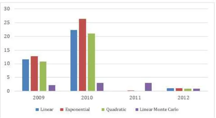
Figure 5. Chart of MSE comparation among regression
Figure 6. Chart of MSE comparation as a result of regression with MSE as result of Monte Carlo linear regression
Bar chart above explain the result of MSE from each regression. The smallest MSE from regression is MSE from linear Monte Carlo regression although in year of 2011, Monte Carlo linear regression is still not good compared to other method but overall result of Monte Carlo linear regression is the best regression compared to another regression.
5.3 Prediction
In order to test Monte Carlo linear regression performance in forecasting, original data paramater from year 2009-2011 that has been performed with missing imputation from three years is combined into one. Data of 2009-2011 is combined into one with name of combined data, those combined data is used for searching function of linear, exponential, quadratic, and linear Monte Carlo regression and data in 2012 is used as validation data for prediction result.
Table 7. Search of regression function in combined data
CH 310 270 600 300 150 120 200 210 500
Kasus (Y) 20 30 15 13 17 25 27 10 10
Table 8. Data year 2012
CH 110 90 200 150 75 0 56 170 250
Kasus (Y) 15 8 5 3 0 5 9 4 0
First table above explains that combined data is searched for the regression fucntion, for example we look for linear regression function and get equation of linear regression function as Y =-0,01242108.x+5,87742. This function is used to calculate data that exist in year 2012. So, x value in linear regression function is filled with case value (Y) in data of 2012. This proccess also is performed on another regression so the next step is calculating MSE to determine the best regression model as prediction. The table below is calculation result of MSE on each regression:
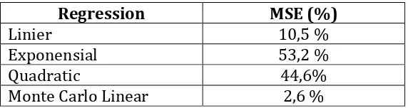
Table 9. MSE comparation among regression
Regression MSE (%)
Linier 10,5 %
Exponensial 53,2 %
Quadratic 44,6%
Monte Carlo Linear 2,6 %
From the table of MSE comparation above, we can know that MSE value from Monte Carlo linear regression is the smallest MSE value. Furthermore, we can see that Monte Carlo linear regression in this prediction has the lowest trend error as compared to linear, exponential, and quadratic regression.
6. CONCLUSION
REFERENCES
[1] Buletin Jendela Epidemiologi. (2010). Demam Berdarah Dengue
(Volume 2). Indonesia: Kementerian Kesehatan.
[2] Wahyu, Sri Yulianto, Identifikasi Missing Value dan Outlier pada
Proses Cleansing Data, 2014, Salatiga.
[3] Han, Jiawei, Micheline Kamber, Jian Pei, Data Mining : Concept and
Techniques, 2011 USA : Morgan Kaufmann.
[4] Nasoetion, Forecasting of Native Chicken Population in Central Java
by Using Trend Least Square Model, 2009 National Seminar
Awakening Ranch, Semarang, 20, 2009.
[5] Achmad Basuki, Miftahul Huda, Tri Budi. Model and Simulation, 2014, IPTAQ Mulia Media, Jakarta.
[6] Addie Andromeda Evans, Maximum Likelihood Estimation, 2008, San Fransisco State University.
[7] Jiaqi Ge, Yuni Xia and Jian Wang, A Na¨ıve Bayesian Classifier in
Categorical Uncertain Data Streams, Indiana University, Purdue
University Indianapolis and Nanjing University.
[8] Gintautas Dzemyda, Leonidas Sakalauskas, Large-Scale Data Analysis
Using Heuristic Methods, INFORMATICA, 2011, Vol. 22, No. 1, 1–10.
[9] H. Abdul Rahiml , F. Ibrahim, A Novel Prediction System In Dengue
Fever Using Narmax Model, International Conference on Control,
Automation and Systems 2007 Oct. 17-20, 2007 in COEX, Seoul, Korea. [10] Napa Rachata, Phasit Charoenkwan, Thongchai Yooyativong, Kosin
Chamnongthal, Chidchanok Lursinsap, and Kohji Higuchi, Automatic Prediction System of Dengue Haemorrhagic-Fever Outbreak Risk
by Using Entropy and Artificial Neural Network, International
Symposium on Communications and Information Technologies (ISCIT 2008).
[11] Dia Bitari Mei Yuana, I Putu Dody Lesmana, Slamet Yulianto, Model Potential Spread of Disease Fever Dengue in Jember Method Using
Fuzzy, Prosiding Conference on Smart-Green Technology in Electrical
and Information Systems. Bali, 14-15 November 2013.
[12] Imam Taufik, and Mada Sanjaya WS,Monte Carlo Simulation in Predicting Epidemics of Dengue dengeu in the district of Sukabumi
Citamiang, Physics Conference Proceedings 1 2012, ISSN 2301-5284.
[13] A. E. Maxwell. Analysing Qualitative Data. 4th Edition. Chapman and