Table of Contents
Apache Hive Essentials Credits
About the Author About the Reviewers www.PacktPub.com
Support files, eBooks, discount offers, and more Why subscribe?
Free access for Packt account holders Preface
What this book covers
What you need for this book Who this book is for
Conventions Reader feedback Customer support
Downloading the example code Errata
Piracy Questions
1. Overview of Big Data and Hive A short history
Introducing big data
Relational and NoSQL database versus Hadoop Batch, real-time, and stream processing
Overview of the Hadoop ecosystem Hive overview
Summary
Installing Hive from vendor packages Starting Hive in the cloud
Using the Hive command line and Beeline The Hive-integrated development environment Summary
3. Data Definition and Description Understanding Hive data types Data type conversions
Hive Data Definition Language Hive database
Hive internal and external tables Hive partitions
Hive buckets Hive views Summary
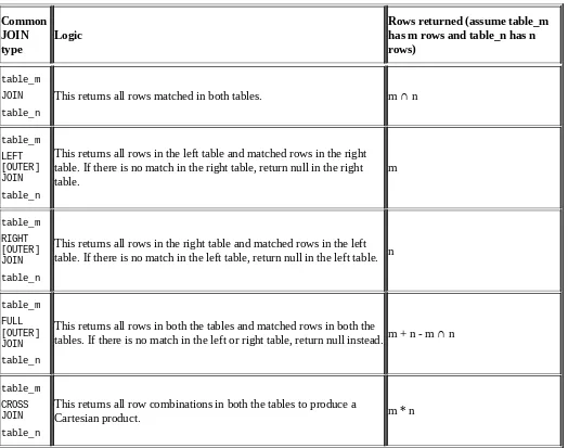
4. Data Selection and Scope The SELECT statement The INNER JOIN statement
The OUTER JOIN and CROSS JOIN statements Special JOIN – MAPJOIN
Set operation – UNION ALL Summary
5. Data Manipulation Data exchange – LOAD Data exchange – INSERT
Data exchange – EXPORT and IMPORT ORDER and SORT
Operators and functions Transactions
Summary
Basic aggregation – GROUP BY
Advanced aggregation – GROUPING SETS Advanced aggregation – ROLLUP and CUBE Aggregation condition – HAVING
Analytic functions Sampling
Summary
7. Performance Considerations Performance utilities
The EXPLAIN statement The ANALYZE statement Design optimization
Partition tables Bucket tables Index
Data file optimization File format
Compression
Storage optimization Job and query optimization
Local mode JVM reuse
Parallel execution Join optimization
Common join Map join
Bucket map join
Sort merge bucket (SMB) join
Sort merge bucket map (SMBM) join Skew join
8. Extensibility Considerations User-defined functions
The UDF code template The UDAF code template The UDTF code template Development and deployment Streaming
SerDe Summary
9. Security Considerations Authentication
Metastore server authentication HiveServer2 authentication Authorization
Legacy mode
Storage-based mode
SQL standard-based mode Encryption
Summary
10. Working with Other Tools JDBC / ODBC connector HBase
Hue HCatalog ZooKeeper Oozie
Apache Hive Essentials
Copyright © 2015 Packt Publishing
All rights reserved. No part of this book may be reproduced, stored in a retrieval system, or transmitted in any form or by any means, without the prior written permission of the publisher, except in the case of brief quotations embedded in critical articles or reviews. Every effort has been made in the preparation of this book to ensure the accuracy of the information presented. However, the information contained in this book is sold without warranty, either express or implied. Neither the author, nor Packt Publishing, and its
dealers and distributors will be held liable for any damages caused or alleged to be caused directly or indirectly by this book.
Packt Publishing has endeavored to provide trademark information about all of the companies and products mentioned in this book by the appropriate use of capitals. However, Packt Publishing cannot guarantee the accuracy of this information. First published: February 2015
Production reference: 1210215 Published by Packt Publishing Ltd. Livery Place
35 Livery Street
Birmingham B3 2PB, UK. ISBN 978-1-78355-857-5
Credits
AuthorDayong Du
Reviewers
Puneetha B M Hamzeh Khazaei Nitin Pradeep Kumar Balaswamy Vaddeman
Commissioning Editor
Ashwin Nair
Acquisition Editor
Shaon Basu
Content Development Editor
Merwyn D’souza
Technical Editor
Taabish Khan
Copy Editors
Sameen Siddiqui Laxmi Subramanian
Project Coordinator
Neha Bhatnagar
Proofreaders
Paul Hindle Jonathan Todd
Indexer
Monica Ajmera Mehta
Production Coordinator
Aparna Bhagat
Cover Work
About the Author
Dayong Du is a big data practitioner, leader, and developer with expertise in technology consulting, designing, and implementing enterprise big data solutions. With more than 10 years of experience in enterprise data warehouse, business intelligence, and big data and analytics, he has provided his data intelligence expertise in various industries, such as media, travel, telecommunications, and so on. He is currently working with QuickPlay Media in Toronto, Canada, to build enterprise big data intelligence reporting for online media services and content providers. He has a master’s degree in computer science from Dalhousie University, and he holds the Cloudera Certified Developer for Apache Hadoop certification.
I would like to sincerely thank my wife, Joice, and daughter, Elaine, for their sacrifices and encouragement during this journey. Also, I would like to thank my parents for their support during the time of writing this book.
About the Reviewers
Puneetha B M is a software engineer, data enthusiast, and technical blogger. Her research interests include big data, cloud computing, machine learning, and NoSQL databases. She is also a professional software engineer with more than 2 years of working experience. She holds a master’s degree in computer applications from P.E.S. Institute of Technology. Other than programming, she enjoys painting and listening to music. You can learn more from her blog (http://blog.puneethabm.in/) and LinkedIn profile
(https://www.linkedin.com/in/puneethabm).
I owe a great deal to Prof. Dr. Ram Rustagi for being a role model in my life and for his zealous inspiration. I would like to thank my brother, Nischith B.M., for supporting me in everything I do. I would also like to thank Packt Publishing and its staff for providing the opportunity to contribute to this book.
Hamzeh Khazaei is a postdoctoral research scientist at IBM Canada Research and
Development Centre. He received his PhD degree in computer science from University of Manitoba, Winnipeg, Manitoba, Canada (2009–2012). Earlier, he received both his BSc and MSc degrees in computer science from Amirkabir University of Technology, Tehran, Iran (2000–2008). He is also a sessional instructor in the Computer Science department at Ryerson University (http://scs.ryerson.ca/~hkhazaei). He teaches software engineering to fourth year undergraduate students. His research area includes big data analytics, cloud computing infrastructure, analytics as a service, and modeling of computing systems. I would like to thank my dear wife for her perpetual support in all my endeavors.
Nitin Pradeep Kumar is a passionate developer with extensive experience and oodles of interest in emerging technologies such as the cloud and mobile. He is currently a cloud quality engineer at Appcelerator, a leading Silicon Valley-based start-up that provides an MBaaS platform purpose-built for mobile and cloud development. Before this stint, he studied at the National University of Singapore toward a master’s degree in knowledge engineering, which involves building intelligent systems using cutting-edge artificial intelligence and data-mining techniques. He enjoys the start-up environment and has worked with technologies such as Hadoop, Hive, and data warehousing. He lives in
Singapore and spends his spare cycles playing retro PC games on his mobile and learning Muay Thai.
I would like to thank my family, friends, and my wonderful brother, Nivin, for supporting me in all my endeavors.
data forums.
Support files, eBooks, discount offers, and
more
For support files and downloads related to your book, please visit www.PacktPub.com. Did you know that Packt offers eBook versions of every book published, with PDF and ePub files available? You can upgrade to the eBook version at www.PacktPub.com and as a print book customer, you are entitled to a discount on the eBook copy. Get in touch with us at <[email protected]> for more details.
At www.PacktPub.com, you can also read a collection of free technical articles, sign up for a range of free newsletters and receive exclusive discounts and offers on Packt books and eBooks.
https://www2.packtpub.com/books/subscription/packtlib
Why subscribe?
Fully searchable across every book published by Packt Copy and paste, print, and bookmark content
Free access for Packt account holders
If you have an account with Packt at www.PacktPub.com, you can use this to access PacktLib today and view 9 entirely free books. Simply use your login credentials for immediate access.
Preface
With an increasing interest in big data analysis, Hive over Hadoop becomes a cutting-edge data solution for storing, computing, and analyzing big data. The SQL-like syntax makes Hive easier to learn and popularly accepted as a standard for interactive SQL queries over big data. The variety of features available within Hive provides us with the capability of doing complex big data analysis without advanced coding skills. The maturity of Hive lets it gradually merge and share its valuable architecture and functionalities across different computing frameworks beyond Hadoop.
What this book covers
Chapter 1, Overview of Big Data and Hive, introduces the evolution of big data, the
Hadoop ecosystem, and Hive. You will also learn the Hive architecture and the advantages of using Hive in big data analysis.
Chapter 2, Setting Up the Hive Environment, describes the Hive environment setup and configuration. It also covers using Hive through the command line and development tools.
Chapter 3, Data Definition and Description, introduces the basic data types and data definition language for tables, partitions, buckets, and views in Hive.
Chapter 4, Data Selection and Scope, shows you ways to discover the data by querying, linking, and scoping the data in Hive.
Chapter 5, Data Manipulation, describes the process of exchanging, moving, sorting, and transforming the data in Hive.
Chapter 6, Data Aggregation and Sampling, explains how to do aggregation and sample using aggregation functions, analytic functions, windowing, and sample clauses.
Chapter 7, Performance Considerations, introduces the best practices of performance considerations in the aspects of design, file format, compression, storage, query, and job.
Chapter 8, Extensibility Considerations, describes how to extend Hive by creating user-defined functions, streaming, serializers, and deserializers.
Chapter 9, Security Considerations, introduces the area of Hive security in terms of authentication, authorization, and encryption.
What you need for this book
You will need to install both Hadoop and Hive to run the examples in this book. The
scripts in this book were written and tested with Cloudera Distributed Hadoop (CDH) v5.3 (contains Hive v0.13.x and Hadoop v2.5.0), Hortonworks Data Platform (HDP) v2.2
(contains Hive v0.14.0 and Hadoop v2.6.0), and Apache Hive 1.0.0 (with Hadoop 1.2.1) in pseudo-distributed mode. However, the majority of the scripts will also run on the previous versions of Hadoop and Hive. The following are the other software applications you may need for a better understanding of the Hive-related tools mentioned in the book. These tools are also available in the CDH or HDP packages.
Hue 2.2.0 and above HBase 0.98.4
Oozie 4.0.0 and above Zookeeper 3.4.5
Who this book is for
Conventions
In this book, you will find a number of text styles that distinguish between different kinds of information. Here are some examples of these styles and an explanation of their
meaning.
Code words in text, database table names, folder names, filenames, file extensions, pathnames, dummy URLs, user input, and Twitter handles are shown as follows: “Aggregate function can be used with other aggregate functions in the same select
statement.”
A block of code is set as follows:
<property>
<name>javax.jdo.option.ConnectionURL</name>
<value>jdbc:mysql://myhost:3306/hive?createDatabase IfNotExist=true</value>
<description>JDBC connect string for a JDBC metastore</description> </property>
When we wish to draw your attention to a particular part of a code block, the relevant lines or items are set in bold:
customAuthenticator.java
package com.packtpub.hive.essentials.hiveudf; import java.util.Hashtable;
import javax.security.sasl.AuthenticationException;
import org.apache.hive.service.auth.PasswdAuthenticationProvider;
Any command-line input or output is written as follows:
bash-4.1$ hdfs dfs –mkdir /tmp
New terms and important words are shown in bold. Words that you see on the screen, for example, in menus or dialog boxes, appear in the text like this: “Click on the OK
button and restart Oracle SQL Developer.”
Note
Warnings or important notes appear in a box like this.
Tip
Reader feedback
Feedback from our readers is always welcome. Let us know what you think about this book—what you liked or disliked. Reader feedback is important for us as it helps us develop titles that you will really get the most out of.
To send us general feedback, simply e-mail <[email protected]>, and mention the
book’s title in the subject of your message.
Customer support
Downloading the example code
You can download the example code files from your account at http://www.packtpub.com
for all the Packt Publishing books you have purchased. If you purchased this book
Errata
Although we have taken every care to ensure the accuracy of our content, mistakes do happen. If you find a mistake in one of our books—maybe a mistake in the text or the code—we would be grateful if you could report this to us. By doing so, you can save other readers from frustration and help us improve subsequent versions of this book. If you find any errata, please report them by visiting http://www.packtpub.com/submit-errata,
selecting your book, clicking on the ErrataSubmissionForm link, and entering the details of your errata. Once your errata are verified, your submission will be accepted and the errata will be uploaded to our website or added to any list of existing errata under the Errata section of that title.
To view the previously submitted errata, go to
Piracy
Piracy of copyrighted material on the Internet is an ongoing problem across all media. At Packt, we take the protection of our copyright and licenses very seriously. If you come across any illegal copies of our works in any form on the Internet, please provide us with the location address or website name immediately so that we can pursue a remedy.
Please contact us at <[email protected]> with a link to the suspected pirated
material.
Questions
If you have a problem with any aspect of this book, you can contact us at
Chapter 1. Overview of Big Data and Hive
This chapter is an overview of big data and Hive, especially in the Hadoop ecosystem. It briefly introduces the evolution of big data so that readers know where they are in the journey of big data and find their preferred areas in future learning. This chapter also covers how Hive has become one of the leading tools in big data warehousing and why Hive is still competitive.
In this chapter, we will cover the following topics:
A short history from database and data warehouse to big data Introducing big data
Relational and NoSQL databases versus Hadoop Batch, real-time, and stream processing
A short history
In the 1960s, when computers became a more cost-effective option for businesses, people started to use databases to manage data. Later on, in the 1970s, relational databases
became more popular to business needs since they connected physical data to the logical business easily and closely. In the next decade, around the 1980s, Structured Query Language (SQL) became the standard query language for databases. The effectiveness and simplicity of SQL motivated lots of people to use databases and brought databases closer to a wide range of users and developers. Soon, it was observed that people used databases for data application and management and this continued for a long period of time.
Once plenty of data was collected, people started to think about how to deal with the old data. Then, the term data warehousing came up in the 1990s. From that time onwards, people started to discuss how to evaluate the current performance by reviewing the historical data. Various data models and tools were created at that time for helping enterprises to effectively manage, transform, and analyze the historical data. Traditional relational databases also evolved to provide more advanced aggregation and analyzed functions as well as optimizations for data warehousing. The leading query language was still SQL, but it was more intuitive and powerful as compared to the previous versions. The data was still well structured and the model was normalized. As we entered the 2000s, the Internet gradually became the topmost industry for the creation of the majority of data in terms of variety and volume. Newer technologies, such as social media analytics, web mining, and data visualizations, helped lots of businesses and companies deal with
massive amounts of data for a better understanding of their customers, products,
competition, as well as markets. The data volume grew and the data format changed faster than ever before, which forced people to search for new solutions, especially from the academic and open source areas. As a result, big data became a hot topic and a
challenging field for many researchers and companies.
However, in every challenge there lies great opportunity. Hadoop was one of the open source projects earning wide attention due to its open source license and active
communities. This was one of the few times that an open source project led to the changes in technology trends before any commercial software products. Soon after, the NoSQL database and real-time and stream computing, as followers, quickly became important components for big data ecosystems. Armed with these big data technologies, companies were able to review the past, evaluate the current, and also predict the future. Around the 2010s, time to market became the key factor for making business competitive and
successful. When it comes to big data analysis, people could not wait to see the reports or results. A short delay could make a great difference when making important business decisions. Decision makers wanted to see the reports or results immediately within a few hours, minutes, or even possibly seconds in a few cases. Real-time analytical tools, such as Impala (
Introducing big data
Big data is not simply a big volume of data. Here, the word “Big” refers to the big scope of data. A well-known saying in this domain is to describe big data with the help of three words starting with the letter V. They are volume, velocity, and variety. But the analytical and data science world has seen data varying in other dimensions in addition to the
fundament 3 Vs of big data such as veracity, variability, volatility, visualization, and value. The different Vs mentioned so far are explained as follows:
Volume: This refers to the amount of data generated in seconds. 90 percent of the world’s data today has been created in the last two years. Since that time, the data in the world doubles every two years. Such big volumes of data is mainly generated by machines, networks, social media, and sensors, including structured, semi-structured, and unstructured data.
Velocity: This refers to the speed in which the data is generated, stored, analyzed, and moved around. With the availability of Internet-connected devices, wireless or wired, machines and sensors can pass on their data immediately as soon as it is created. This leads to real-time streaming and helps businesses to make valuable and fast decisions.
Variety: This refers to the different data formats. Data used to be stored as text, dat, and csv from sources such as filesystems, spreadsheets, and databases. This type of data that resides in a fixed field within a record or file is called structured data.
Nowadays, data is not always in the traditional format. The newer semi-structured or unstructured forms of data can be generated using various methods such as e-mails, photos, audio, video, PDFs, SMSes, or even something we have no idea about. These varieties of data formats create problems for storing and analyzing data. This is one of the major challenges we need to overcome in the big data domain.
Veracity: This refers to the quality of data, such as trustworthiness, biases, noise, and abnormality in data. Corrupt data is quite normal. It could originate due to a number of reasons, such as typos, missing or uncommon abbreviation, data reprocessing, system failures, and so on. However, ignoring this malicious data could lead to
inaccurate data analysis and eventually a wrong decision. Therefore, making sure the data is correct in terms of data audition and correction is very important for big data analysis.
Variability: This refers to the changing of data. It means that the same data could have different meanings in different contexts. This is particularly important when carrying out sentiment analysis. The analysis algorithms are able to understand the context and discover the exact meaning and values of data in that context.
Volatility: This refers to how long the data is valid and stored. This is particularly important for real-time analysis. It requires a target scope of data to be determined so that analysts can focus on particular questions and gain good performance out of the analysis.
comprehensible in a multidimensional view that is easy to understand. Visualization is an innovative way to show changes in data. It requires lots of interaction,
conversations, and joint efforts between big data analysts and business domain experts to make the visualization meaningful.
Value: This refers to the knowledge gained from data analysis on big data. The value of big data is how organizations turn themselves into big data-driven companies and use the insight from big data analysis for their decision making.
Relational and NoSQL database versus
Hadoop
Let’s compare different data solutions with the ways of traveling. You will be surprised to find that they have many similarities. When people travel, they either take cars or
airplanes depending on the travel distance and cost. For example, when you travel to Vancouver from Toronto, an airplane is always the first choice in terms of the travel time versus cost. When you travel to Niagara Falls from Toronto, a car is always a good choice. When you travel to Montreal from Toronto, some people may prefer taking a car to an airplane. The distance and cost here is like the big data volume and investment. The traditional relational database is like the car in this example. The Hadoop big data tool is like the airplane in this example. When you deal with a small amount of data (short
distance), a relational database (like the car) is always the best choice since it is more fast and agile to deal with a small or moderate size of data. When you deal with a big amount of data (long distance), Hadoop (like the airplane) is the best choice since it is more linear, fast, and stable to deal with the big size of data. On the contrary, you can drive from
Toronto to Vancouver, but it takes too much time. You can also take an airplane from Toronto to Niagara, but it could take more time and cost way more than if you travel by a car. In addition, you may have a choice to either take a ship or a train. This is like a
Batch, real-time, and stream processing
Batch processing is used to process data in batches and it reads data input, processes it, and writes it to the output. Apache Hadoop is the most well-known and popular open source implementation of batch processing and a distributed system using the MapReduce paradigm. The data is stored in a shared and distributed filesystem called HadoopDistributed File System (HDFS), divided into splits, which are the logical data divisions for MapReduce processing. To process these splits using the MapReduce paradigm, the map task reads the splits and passes all of its key/value pairs to a map function and writes the results to intermediate files. After the map phase is completed, the reducer reads intermediate files and passes it to the reduce function. Finally, the reduce task writes results to the final output files. The advantages of the MapReduce model include making distributed programming easier, near-linear speed up, good scalability, as well as fault tolerance. The disadvantage of this batch processing model is being unable to execute recursive or iterative jobs. In addition, the obvious batch behavior is that all inputs must be ready by map before the reduce job starts, which makes MapReduce unsuitable for online and stream processing use cases.
Real-time processing is to process data and get the result almost immediately. This concept in the area of real-time ad hoc queries over big data was first implemented in Dremel by Google. It uses a novel columnar storage format for nested structures with fast index and scalable aggregation algorithms for computing query results in parallel instead of batch sequences. These two techniques are the major characters for real-time processing and are used by similar implementations, such as Cloudera Impala, Facebook Presto,
Apache Drill, and Hive on Tez powered by Stinger whose effort is to make a 100x
performance improvement over Apache Hive. On the other hand, in-memory computing no doubt offers other solutions for real-time processing. In-memory computing offers very high bandwidth, which is more than 10 gigabytes/second, compared to hard disks’ 200 megabytes/second. Also, the latency is comparatively lower, nanoseconds versus
milliseconds, compared to hard disks. With the price of RAM going lower and lower each day, in-memory computing is more affordable as real-time solutions, such as Apache Spark, which is a popular open source implementation of in-memory computing. Spark can be easily integrated with Hadoop and the resilient distributed dataset can be generated from data sources such as HDFS and HBase for efficient caching.
Stream processing is to continuously process and act on the live stream data to get a result. In stream processing, there are two popular frameworks: Storm
(https://storm.apache.org/) from Twitter and S4 (http://incubator.apache.org/s4/) from Yahoo!. Both the frameworks run on the Java Virtual Machine (JVM) and both process keyed streams. In terms of the programming model, S4 is a program defined as a graph of
Overview of the Hadoop ecosystem
Hadoop was first released by Apache in 2011 as version 1.0.0. It only contained HDFS and MapReduce. Hadoop was designed as both a computing (MapReduce) and storage (HDFS) platform from the very beginning. With the increasing need for big data analysis, Hadoop attracts lots of other software to resolve big data questions together and merges to a Hadoop-centric big data ecosystem. The following diagram gives a brief introduction to the Hadoop ecosystem and the core software or components in the ecosystems:
The Hadoop ecosystem
In the current Hadoop ecosystem, HDFS is still the major storage option. On top of it, snappy, RCFile, Parquet, and ORCFile could be used for storage optimization. Core Hadoop MapReduce released a version 2.0 called Yarn for better performance and
scalability. Spark and Tez as solutions for real-time processing are able to run on the Yarn to work with Hadoop closely. HBase is a leading NoSQL database, especially when there is a NoSQL database request on the deployed Hadoop clusters. Sqoop is still one of the leading and matured tools for exchanging data between Hadoop and relational databases.
Flume is a matured distributed and reliable log-collecting tool to move or collect data to HDFS. Impala and Presto query directly against the data on HDFS for better
Hive overview
Hive is a standard for SQL queries over petabytes of data in Hadoop. It provides SQL-like access for data in HDFS making Hadoop to be used like a warehouse structure. The Hive Query Language (HQL) has similar semantics and functions as standard SQL in the relational database so that experienced database analysts can easily get their hands on it. Hive’s query language can run on different computing frameworks, such as MapReduce, Tez, and Spark for better performance.
Hive’s data model provides a high-level, table-like structure on top of HDFS. It supports three data structures: tables, partitions, and buckets, where tables correspond to HDFS directories and can be divided into partitions, which in turn can be divided into buckets. Hive supports a majority of primitive data formats such as TIMESTAMP, STRING, FLOAT, BOOLEAN, DECIMAL, DOUBLE, INT, SMALLINT, BIGINT, and complex data types, such as UNION, STRUCT, MAP, and ARRAY.
The following diagram is the architecture seen inside the view of Hive in the Hadoop ecosystem. The Hive metadata store (or called metastore) can use either embedded, local, or remote databases. Hive servers are built on Apache Thrift Server technology. Since Hive has released 0.11, Hive Server 2 is available to handle multiple concurrent clients, which support Kerberos, LDAP, and custom pluggable authentication, providing better options for JDBC and ODBC clients, especially for metadata access.
Hive architecture
Here are some highlights of Hive that we can keep in mind moving forward: Hive provides a simpler query model with less coding than MapReduce HQL and SQL have similar syntax
Hive provides lots of functions that lead to easier analytics usage
type of huge datasets
Hive supports running on different computing frameworks Hive supports ad hoc querying data on HDFS
Hive supports user-defined functions, scripts, and a customized I/O format to extend its functionality
Hive is scalable and extensible to various types of data and bigger datasets
Matured JDBC and ODBC drivers allow many applications to pull Hive data for seamless reporting
Hive allows users to read data in arbitrary formats, using SerDes and Input/Output formats
Hive has a well-defined architecture for metadata management, authentication, and query optimizations
Summary
After going through this chapter, we are now able to understand why and when to use big data instead of a traditional relational database. We also understand the difference between batch processing, real-time processing, and stream processing. We got familiar with the Hadoop ecosystem, especially Hive. We have also gone back in time and brushed through the history of database and warehouse to big data along with some big data terms, the Hadoop ecosystem, Hive architecture, and the advantage of using Hive. In the next
Chapter 2. Setting Up the Hive
Environment
This chapter will introduce how to install and set up the Hive environment in the cluster and cloud. It also covers the usage of basic Hive commands and the Hive-integrated development environment.
In this chapter, we will cover the following topics: Installing Hive from Apache
Installing Hive from vendor packages Starting Hive in the cloud
Installing Hive from Apache
To introduce the Hive installation, we use Hive version 1.0.0 as an example. The pre-installation requirements for this pre-installation are as follows:
JDK 1.7.0_51
Hadoop 0.20.x, 0.23.x.y, 1.x.y, or 2.x.y Ubuntu 14.04/CentOS 6.2
Note
Since we focus on Hive in this book, the installation steps for Java and Hadoop are not provided here. For steps on installing them, please refer to
https://www.java.com/en/download/help/download_options.xml and
http://hadoop.apache.org/docs/current/hadoop-project-dist/hadoop-common/ClusterSetup.html.
The following steps describe how to install Hive from Apache through the Linux command line:
1. Download Hive from Apache Hive and unpack it:
bash-4.1$ wget
http://apache.mirror.rafal.ca/hive/hive-1.0.0/apache-3. Enable the settings immediately:
bash-4.1$ source /etc/profile
4. Create the configuration files:
bash-4.1$ cd apache-hive-1.0.0-bin/conf
5. Modify the configuration file at $HIVE_HOME/conf/hive-env.sh:
#Set HADOOP_HOME to point to a specific Hadoop install directory export HADOOP_HOME=/home/hivebooks/hadoop-2.2.0
#Hive Configuration Directory can be accessed at:
export HIVE_CONF_DIR=/home/hivebooks/apache-hive-1.0.0-bin/conf
6. Modify the configuration file at $HIVE_HOME/conf/hive-site.xml. There are some
hive.metastore.warehourse.dir: This is the path for Hive warehouse storage.
By default it is /user/hive/warehouse.
hive.exec.scratchdir: This is the temporary data file path. By default it is /tmp/hive-${user.name}.
By default, Hive uses the Derby (http://db.apache.org/derby/) database as the metadata store. Hive can also use other databases, such as PostgreSQL (http://www.postgresql.org/) or MySQL (http://www.mysql.com/) as the metadata store. To configure Hive to use other databases, the following parameters should be configured:
javax.jdo.option.ConnectionURL // the database URL javax.jdo.option.ConnectionDriverName // the JDBC driver name javax.jdo.option.ConnectionUserName // database username javax.jdo.option.ConnectionPassword // database password
The following is an example setting using MySQL as the metastore database:
<property>
<name>javax.jdo.option.ConnectionURL</name>
<value>jdbc:mysql://myhost:3306/hive?createDatabase IfNotExist=true</value>
<description>JDBC connect string for a JDBC metastore</description> </property>
<property>
<name>javax.jdo.option.ConnectionDriverName</name> <value>com.mysql.jdbc.Driver</value>
<description>Driver class name for a JDBC metastore</description> </property>
<property>
<name>javax.jdo.option.ConnectionUserName</name> <value>hive</value>
<description>username to use against metastore database</description> </property>
<property>
<name>javax.jdo.option.ConnectionPassword</name> <value>hive</value>
<description>password to use against metastore database</description> </property>
Make sure the MySQL JDBC driver is available at $HIVE_HOME/lib.
Note
The differences between an embed Derby database and an external database is that an external database offers a shared service so that users can share the metadata of Hive. However, an embed database is only visible to the local users.
Create folders and grant proper write permissions to the user group in the HDFS folder:
bash-4.1$ hdfs dfs –mkdir /tmp
bash-4.1$ hdfs dfs –mkdir /user/hive/warehouse bash-4.1$ hdfs dfs -chmod g+w /tmp
That’s all about Apache Hive installation. In one of the Hive nodes installed, type hive to
enter the Hive command-line environment (hive>), which verifies Hive is successfully
Installing Hive from vendor packages
Right now, many companies, such as Cloudera, MapR, IBM, and Hortonworks, have packaged Hadoop into more easily manageable distributions. Each company takes a slightly different strategy, but the consensus for all of these packages is to make Hadoop easier to use for enterprise. For example, we can easily install Hive from Cloudera Distributed Hadoop (CDH), which can be downloaded from
http://www.cloudera.com/content/cloudera/en/downloads/cdh.html.
Once CDH is installed to have the Hadoop environment ready, we can add Hive to the Hadoop cluster by following a few steps:
1. Log in to the Cloudera manager and click on the dropdown button after the cluster name to choose Add a Service.
Cloudera manager main page
3. In the second Add Service Wizard page, set the dependencies for the service.
Sentry is the authorization policy service for Hive.
4. In the third Add Service Wizard page, choose the proper hosts for HiveServer2, Hive Metastore Server, WebHCat Server, and Gateway.
6. In the last page of Add Service Wizard, review the changes on the Hive warehouse directory and metastore server port number. Keep the default values and click on the
Continue button to start installing the Hive service. Once it is complete, close the wizard to finish the Hive installation.
Note
Starting Hive in the cloud
Right now, Amazon EMR, Cloudera Director, and Microsoft Azure HDInsight Service are some of the major vendors offering matured Hadoop and Hive services in the cloud. Using the cloud version of Hive is very convenient. It almost requests no installation and setup. Amazon EMR (http://aws.amazon.com/elasticmapreduce/) is the earliest Hadoop service in the cloud. However, it is not a pure open sourced version of Hadoop, but is customized to run only on AWS cloud. Cloudera is one of the first few players that offered open
source Hadoop solutions to the enterprise. Since the middle of October 2014, Cloudera has delivered Cloudera Director ( http://www.cloudera.com/content/cloudera/en/products-and-services/director.html), which opens up Hadoop deployments in the cloud through a
simple, self-service interface, and is fully supported on Amazon Web Services. Windows Azure HDInsight Service (
http://azure.microsoft.com/en-us/documentation/services/hdinsight/) is a service that deploys and provisions Apache Hadoop clusters in the Azure cloud. Although Hadoop was first built on Linux,
Hortonworks and Microsoft have partnered to bring the benefits of Apache Hadoop to the Windows Azure cloud.
Using the Hive command line and Beeline
Hive first started with HiveServer1. However, this version of the Hive server was not very stable. It sometimes suspended or blocked clients’ connection quietly. Since version 11, Hive includes a new Hive server called HiveSever2 as an addition to HiveServer1. HiveServer2 is an enhanced Hive server designed for multiclient concurrency and
improved authentication. HiveServer2 also supports Beeline as the alternative command-line interface. HiveServer1 is deprecated and removed from Hive since version 1.0.0. The primary difference between the two Hive servers is how the clients connect to Hive. Hive CLI is an Apache Thrift-based client, and Beeline is a JDBC client based on
SQLLine (http://sqlline.sourceforge.net/) CLI. The Hive CLI directly connects to the Hive drivers and requires installing Hive on the same machine as the client. However, Beeline connects to HiveServer2 through JDBC connections and does not require the installation of Hive libraries on the same machine as the client. That means we can run Beeline remotely from outside of the Hadoop cluster.
The following table is the commonly used commands for both Beeline and Hive CLI. For more usage of HiveServer2 and Beeline, refer to
https://cwiki.apache.org/confluence/display/Hive/HiveServer2+Clients.
Purpose HiveServer2 Beeline HiveServer1 CLI
Server connection beeline –u <jdbcurl> -n <username> -p <password> hive -h <hostname> -p <port>
Help beeline -h or beeline --help hive -H
Run query beeline -e <query in quotes>beeline -f <query file name> hive -e <query in quotes>hive -f <query file name>
Define variable beeline --hivevar key=value.
This is available after Hive 0.13.0. hive --hivevar key=value
The following is the command-line syntax in Beeline or Hive CLI:
Purpose HiveServer2 Beeline HiveServer1 CLI
Enter mode beeline hive
Connect !connect <jdbcurl> n/a
List tables !table show tables;
List columns !column <table_name> desc <table_name>;
Run query <HQL query>; <HQL query>;
Run shell CMD !sh ls
This is available since Hive 0.14.0. !ls;
Run dfs CMD dfs -ls dfs -ls;
Run file of SQL !run <file_name> source <file_name>;
Check Hive version !dbinfo !hive --version;
Quit mode !quit quit;
Note
For Beeline, ; is not needed after the command that starts with !.
When running a query in Hive CLI, the MapReduce statistics information is shown in the console screen while processing, whereas Beeline does not.
Both Beeline and Hive CLI do not support running a pasted query with <tab> inside, because <tab> is used for autocomplete by default in the environment. Alternatively, running the query from files has no such issues.
Hive CLI shows the exact line and position of the Hive query or syntax errors when the query has multiple lines. However, Beeline processes the multiple-line query as a single line, so only the position is shown for query or syntax errors with the line number as 1 for all instances. For this aspect, Hive CLI is more convenient than Beeline for debugging the Hive query.
In both Hive CLI and Beeline, using the up and down arrow keys can retrieve up to 10,000 previous commands. The !history command can be used in Beeline to show all history.
Both Hive CLI and Beeline supports variable substitution; refer to
https://cwiki.apache.org/confluence/display/Hive/LanguageManual+VariableSubstitution. A list of Hive configuration settings and properties can be accessed and overwritten by the
set keyword from the command-line environment. For more details, refer to the Apache
The Hive-integrated development
environment
Besides the command-line interface, there are a few integrated development
environment (IDE) tools available for Hive development. One of the best is Oracle SQL Developer, which leverages the powerful functionalities of Oracle IDE and is totally free to use. If we have to use Oracle along with Hive in a project, it is quite convenient to switch between them only from the same IDE.
Oracle SQL developer has supported Hive since version 4.0.3. Configuring it to work with Hive is quite straightforward. The following are a few steps to configure the IDE to
connect to Hive:
1. Download Hive JDBC drivers from the vendor website, such as Cloudera. 2. Unzip the JDBC version 4 driver to a local directory.
3. Start Oracle SQL Developer and navigate to Preferences | Database | Third Party JDBC Drivers.
4. Add all of the JAR files contained in the unzipped directory to the Third-party JDBC Driver Path setting as follows:
SQL developer configuration
5. Click on the OK button and restart Oracle SQL Developer.
Username, Password, Host name (Hive server hostname), Port, and Database. Then, click on the Add and Connect buttons to connect to Hive.
SQL developer connections
In Oracle SQL Developer, we can run all Hive interactive commands as well as Hive queries. We can also leverage the power of Oracle SQL Developer to browse and export data into a Hive table from the graphic user interface and wizard.
Besides Hive IDE, Hive also has its own built-in web interface, HiveWebInterface. However, it is not powerful and is not being used very often. Hue (http://gethue.com/) is another web interface for the Hadoop ecosystem, including Hive. It is a very powerful and user-friendly web user interface. More details about using Hue with Hive are introduced in
Summary
In this chapter, we introduced the setup of Hive in different environments with proper settings. We also looked into a few of the Hive interactive commands and queries in Hive CLI, Beeline, and IDEs. After going through this chapter, we should be able to set up our own Hive environment locally and use Hive from CLI or IDE tools.
Chapter 3. Data Definition and
Description
This chapter introduces the basic data types, data definition language, and schema in Hive to describe data. It also covers the best practices to describe data correctly and effectively by using internal or external tables, partitions, buckets, and views.
In this chapter, we will cover the following topics: Hive primitive and complex data types
Data type conversions Hive tables
Understanding Hive data types
Hive data types are categorized into two types: primitive and complex data types. String and integer are the most useful primitive types, which are supported by most Hive
functions.
Tip
Downloading the example code
You can download the example code files from your account at http://www.packtpub.com
for all the Packt Publishing books you have purchased. If you purchased this book
elsewhere, you can visit http://www.packtpub.com/support and register to have the files e-mailed directly to you
The details of primitive types are as follows:
Primitive
data type Description Example
TINYINT It has 1 byte from -128 to 127. The postfix is Y. It is used as a small range of
numbers. 10Y
SMALLINT It has 2 bytes from -32,768 to 32,767. The postfix is S. It is used as a regular
descriptive number. 10S
INT It has 4 bytes from -2,147,483,648 to 2,147,483,647. 10
BIGINT It has 8 bytes from -9,223,372,036,854,775,808 to 9,223,372,036,854,775,807. The
postfix is L. 100L
FLOAT
This is a 4-byte single precision floating point number from
1.40129846432481707e-45 to 3.40282346638528860e+38 (positive or negative). Scientific notation is not yet supported. It stores very close approximations of numeric values.
1.2345679
DOUBLE
This is an 8-byte double precision floating point number from
4.94065645841246544e-324d to 1.79769313486231570e+308d (positive or negative). Scientific notation is not yet supported. It stores very close approximations of numeric values.
1.2345678901234567
DECIMAL
This was introduced in Hive 0.11.0 with a hardcode precision of 38 digits. Hive 0.13.0 introduced user definable precision and scale. It is around 1039 - 1 to 1 - 1038. Decimal data types store exact representations of numeric values. The default definition of this type is decimal(10,0).
DECIMAL (3,2) for 3.14
BINARY This was introduced in Hive 0.8.0 and only supports CAST to STRING and vice versa. 1011
BOOLEAN This is a TRUE or FALSE value. TRUE
STRING This includes characters expressed with either single quotes (‘) or double quotes (“).
CHAR This is available starting with Hive 0.13.0. Most UDF will work for this type after
Hive 0.14.0. The maximum length is fixed at 255. ‘US’ or “US”
VARCHAR
This is available starting with Hive 0.12.0. Most UDF will work for this type after Hive 0.14.0. The maximum length is fixed at 65355. If a string value being converted/assigned to a varchar value exceeds the length specified, the string is silently truncated.
‘Books’ or “Books”
DATE This describes a specific year, month, and day in the format of YYYY-MM-DD. It is
available since Hive 0.12.0. The range of date is from 0000-01-01 to 9999-12-31. ‘2013-01-01’
TIMESTAMP This describes a specific year, month, day, hours, minutes, seconds, andmilliseconds in the format of YYYY-MM-DD HH:MM:SS[.fff…]. It is available
since Hive 0.8.0.
‘2013-01-01 12:00:01.345’
Hive has three main complex types: ARRAY, MAP, and STRUCT. These data types are built on
top of the primitive data types. ARRAY and MAP are similar to that in Java. STRUCT is a
record type, which may contain a set of any type of fields. Complex types allow the nesting of types. The details of complex types are as follows:
Complex data
type Description Example
ARRAY This is a list of items of the same type, such as (val1, val2, and so on). You can
access the value using array_name[index], for example, fruit[0]='apple'. [‘apple’,‘orange’,‘mango’]
MAP This is a set of key-value pairs, such as (key1, val1, key2, val2, and so on). You
can access the value using map_name[key], for example, fruit[1]="apple". {1: “apple”,2: “orange”}
STRUCT
This is a user-defined structure of any type of fields, such as {val1, val2, val3, and so on}. By default, STRUCT field names will be col1, col2, and so on. You
can access the value using structs_name.column_name, for example, fruit.col1=1.
{1, “apple”}
NAMED STRUCT
This is a user-defined structure of any number of typed fields, such as (name1, val1, name2, val2, and so on). You can access the value using
structs_name.column_name, for example, fruit.apple="gala".
{“apple”:“gala”,“weight kg”:1}
UNION This is a structure that has exactly any one of the specified data types. It is
available since Hive 0.7.0. It is not commonly used. {2:[“apple”,“orange”]}
Note
For MAP, the type of keys and values are unified. However, STRUCT is more flexible. STRUCT is more like a table whereas MAP is more like an ARRAY with a customized index.
The following is a short practice for all the commonly used Hive types. The details of the
CREATE, LOAD, and SELECT statements will be described later. Let’s take a look at the
process:
1. Prepare the data as follows:
Michael|Montreal,Toronto|Male,30|DB:80|Product:Developer^DLead Will|Montreal|Male,35|Perl:85|Product:Lead,Test:Lead
Shelley|New York|Female,27|Python:80|Test:Lead,COE:Architect Lucy|Vancouver|Female,57|Sales:89,HR:94|Sales:Lead
2. Log in to Beeline with the proper HiveServer2 hostname, port number, database name, username, and password:
-bash-4.1$ beeline
beeline> !connect jdbc:hive2://localhost:10000/default scan complete in 20ms Connecting to
jdbc:hive2://localhost:10000/default
Enter username for jdbc:hive2://localhost:10000/default:dayongd Enter password for jdbc:hive2://localhost:10000/default:
. . . .> sex_age STRUCT<sex:string,age:int>, . . . .> skills_score MAP<string,int>,
. . . .> depart_title MAP<string,ARRAY<string>> . . . .> )
. . . .> ROW FORMAT DELIMITED . . . .> FIELDS TERMINATED BY '|'
. . . .> COLLECTION ITEMS TERMINATED BY ',' . . . .> MAP KEYS TERMINATED BY ':';
No rows affected (0.149 seconds)
4. Verify the table’s creation:
jdbc:hive2://>!table employee
+---+---+---+---+---+ |TABLE_CAT|TABLE_SCHEMA| TABLE_NAME | TABLE_TYPE | REMARKS | +---+---+---+---+---+
| default | employee | depart_title | map<string,array<string>> |
+---+---+---+---+
5. Load data into the table:
No rows affected (1.023 seconds)
6. Query all the rows in the table:
jdbc:hive2://> SELECT * FROM employee;
+---+---+---+---+---4 rows selected (0.677 seconds)
7. Query the whole array and each array column in the table:
jdbc:hive2://> SELECT work_place FROM employee; +---+
| work_place | +---+ | [Montreal, Toronto] | | [Montreal] | | [New York] | | [Vancouver] | +---+
4 rows selected (27.231 seconds)
jdbc:hive2://> SELECT work_place[0] AS col_1,
. . . .> work_place[1] AS col_2, work_place[2] AS col_3 4 rows selected (24.689 seconds)
8. Query the whole struct and each struct column in the table:
jdbc:hive2://> SELECT sex_age FROM employee; +---+
| [Female, 27] | | [Female, 57] | +---+
4 rows selected (28.91 seconds)
jdbc:hive2://> SELECT sex_age.sex, sex_age.age FROM employee; +---+---+
4 rows selected (26.663 seconds)
9. Query the whole map and each map column in the table:
jdbc:hive2://> SELECT skills_score FROM employee; +---+
4 rows selected (32.659 seconds)
jdbc:hive2://> SELECT name, skills_score['DB'] AS DB, . . . .> skills_score['Perl'] AS Perl, 4 rows selected (24.669 seconds)
Note
Note that the column name shown in the result set for Hive is always in lowercase letters.
10. Query the composite type in the table:
jdbc:hive2://> SELECT depart_title FROM employee; +---+
| {Test=[Lead], Product=[Lead]} | | {Test=[Lead], COE=[Architect]} | | {Sales=[Lead]} | +---+ 4 rows selected (30.583 seconds)
jdbc:hive2://> SELECT name, 4 rows selected (26.641 seconds)
jdbc:hive2://> SELECT name,
. . . .> depart_title['Product'][0] AS product_col0, . . . .> depart_title['Test'][0] AS test_col0 4 rows selected (26.659 seconds)
Note
The default delimiters in Hive are as follows:
Row delimiter: This can be used with Ctrl + A or ^A (Use \001 when creating the
table)
Collection item delimiter: This can be used with Ctrl + B or ^B (\002) Map key delimiter: This can be used with Ctrl + C or ^C (\003)
If the delimiter is overidden during the table creation, it only works when used in the flat structure. This is still a limitation in Hive described in Apache Jira Hive-365
(https://issues.apache.org/jira/browse/HIVE-365).
For nested types, for example, the depart_title column in the preceding tables, the level
of nesting determines the delimiter. Using ARRAY of ARRAY as an example, the delimiters
for the outer ARRAY are Ctrl + B (\002) characters, as expected, but for the inner ARRAY they
Data type conversions
Similar to Java, Hive supports both implicit type conversion and explicit type conversion. Primitive type conversion from a narrow to a wider type is known as implicit conversion. However, the reverse conversion is not allowed. All the integral numeric types, FLOAT, and STRING can be implicitly converted to DOUBLE, and TINYINT, SMALLINT, and INT can all be
converted to FLOAT. BOOLEAN types cannot be converted to any other type. In the Apache
Hive wiki, there is a data type cross table describing the allowed implicit conversion between every two types in Hive and this can be found at
https://cwiki.apache.org/confluence/display/Hive/LanguageManual+Types.
Explicit type conversion is using the CAST function with the CAST(value AS TYPE) syntax.
For example, CAST('100' AS INT) will convert the string 100 to the integer value 100. If
Hive Data Definition Language
Hive Data Definition Language (DDL) is a subset of Hive SQL statements that describe the data structure in Hive by creating, deleting, or altering schema objects such as
databases, tables, views, partitions, and buckets. Most Hive DDL statements start with the keywords CREATE, DROP, or ALTER. The syntax of Hive DDL is very similar to the DDL in
Hive database
The database in Hive describes a collection of tables that are used for a similar purpose or belong to the same groups. If the database is not specified, the default database is used. Whenever a new database is created, Hive creates a directory for each database at
/user/hive/warehouse, defined in hive.metastore.warehouse.dir. For example, the myhivebook database is located at /user/hive/datawarehouse/myhivebook.db.
However, the default database doesn’t have its own directory. The following is the core DDL for Hive databases:
Create the database without checking whether the database already exists:
jdbc:hive2://> CREATE DATABASE myhivebook;
Create the database and check whether the database already exists:
jdbc:hive2://> CREATE DATABASE IF NOT EXISTS myhivebook;
Create the database with location, comments, and metadata information:
jdbc:hive2://> CREATE DATABASE IF NOT EXISTS myhivebook . . . .> COMMENT 'hive database demo'
. . . .> LOCATION '/hdfs/directory'
. . . .> WITH DBPROPERTIES ('creator'='dayongd','date'='2015-01-01');
Show and describe the database with wildcards:
jdbc:hive2://> SHOW DATABASES;
1 row selected (1.7 seconds)
jdbc:hive2://> SHOW DATABASES LIKE 'my.*'; jdbc:hive2://> DESCRIBE DATABASE default; 1 row selected (1.352 seconds)
Use the database:
jdbc:hive2://> USE myhivebook;
Drop the empty database:
jdbc:hive2://> DROP DATABASE IF EXISTS myhivebook;
Note that Hive keeps the database and the table in directory mode. In order to remove the parent directory, we need to remove the subdirectories first. By default, the
database cannot be dropped if it is not empty, unless CASCADE is specified. CASCADE
drops the tables in the database automatically before dropping the database. Drop the database with CASCADE:
jdbc:hive2://> DROP DATABASE IF EXISTS myhivebook CASCADE;
Alter the database properties. The ALTER DATABASE statement can only apply to the
table properties and roles (Hive 0.13.0 and later) on the table. The other metadata about the database cannot be changed:
jdbc:hive2://> ALTER DATABASE myhivebook
. . . .> SET DBPROPERTIES ('edited-by' = 'Dayong');
jdbc:hive2://> ALTER DATABASE myhivebook SET OWNER user dayongd;
Note
SHOW and DESCRIBE
The SHOW and DESCRIBE keywords in Hive are used to show the definition information for
most of the Hive objects, such as tables, partitions, and so on.
The SHOW statement supports a wide range of Hive objects, such as tables, tables’
properties, table DDL, index, partitions, columns, functions, locks, roles, configurations, transactions, and compactions.
The DESCRIBE statement supports a small range of Hive objects, such as databases, tables,
views, columns, and partitions. However, the DESCRIBE statement is able to provide more
detailed information combined with the EXTENDED or FORMATTED keywords.
In this book, there is no single section to introduce SHOW and DESCRIBE, but we introduce
Hive internal and external tables
The concept of a table in Hive is very similar to the table in the relational database. Each table associates with a directory configured in ${HIVE_HOME}/conf/hive-site.xml in
HDFS. By default, it is /user/hive/warehouse in HDFS. For example,
/user/hive/warehouse/employee is created by Hive in HDFS for the employee table. All
the data in the table will be kept in the directory. The Hive table is also referred to as internal or managed tables.
When there is data already in HDFS, an external Hive table can be created to describe the data. It is called EXTERNAL because the data in the external table is specified in the
LOCATION properties instead of the default warehouse directory. When keeping data in the
internal tables, Hive fully manages the life cycle of the table and data. This means the data is removed once the internal table is dropped. If the external table is dropped, the table metadata is deleted but the data is kept. Most of the time, an external table is preferred to avoid deleting data along with tables by mistake. The following are DDLs for Hive internal and external table examples:
Show the database file’s location and content of the employee internal table:
bash-4.1$ vi /home/hadoop/employee.txt
Michael|Montreal,Toronto|Male,30|DB:80|Product:Developer^DLead Will|Montreal|Male,35|Perl:85|Product:Lead,Test:Lead
Shelley|New York|Female,27|Python:80|Test:Lead,COE:Architect Lucy|Vancouver|Female,57|Sales:89,HR:94|Sales:Lead
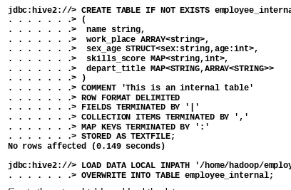
Create the internal table and load the data:
jdbc:hive2://> CREATE TABLE IF NOT EXISTS employee_internal . . . .> (
. . . .> name string,
. . . .> work_place ARRAY<string>,
. . . .> sex_age STRUCT<sex:string,age:int>, . . . .> skills_score MAP<string,int>,
. . . .> depart_title MAP<STRING,ARRAY<STRING>> . . . .> ) No rows affected (0.149 seconds)
jdbc:hive2://> LOAD DATA LOCAL INPATH '/home/hadoop/employee.txt' . . . .> OVERWRITE INTO TABLE employee_internal;
Create the external table and load the data:
jdbc:hive2://> CREATE EXTERNAL TABLE employee_external . . . .> (
. . . .> name string,
. . . .> sex_age STRUCT<sex:string,age:int>, . . . .> skills_score MAP<string,int>,
. . . .> depart_title MAP<STRING,ARRAY<STRING>> . . . .> )
. . . .> LOCATION '/user/dayongd/employee'; No rows affected (1.332 seconds)
jdbc:hive2://> LOAD DATA LOCAL INPATH '/home/hadoop/employee.txt'. . . . . . .> OVERWRITE
INTO TABLE employee_external;
Note
CREATE TABLE
The Hive table does not have constraints such as a database yet.
If the folder in the path does not exist in the LOCATION property, Hive will create that
folder. If there is another folder inside the folder specified in the LOCATION property,
Hive will NOT report errors when creating the table, but will report an error when querying the table.
A temporary table, which is automatically deleted at the end of the Hive session, is supported in Hive 0.14.0 by HIVE-7090 ( https://issues.apache.org/jira/browse/HIVE-7090) through the CREATE TEMPORARY TABLE statement.
For the STORE AS property, it is set to AS TEXTFILE by default. Other file format
values, such as SEQUENCEFILE, RCFILE, ORC, AVRO (since Hive 0.14.0), and PARQUET
(since Hive 0.13.0) can also be specified. Create the table as select (CTAS):
jdbc:hive2://> CREATE TABLE ctas_employee
. . . .> AS SELECT * FROM employee_external; No rows affected (1.562 seconds)
Note
CTAS
CTAS copies the data as well as table definitions. The table created by CTAS is atomic;
this means that other users do not see the table until all the query results are populated. CTAS has the following restrictions:
The table created cannot be a partitioned table The table created cannot be an external table The table created cannot be a list bucketing table
does not trigger any MapReduce job.
CTAS with Common Table Expression (CTE) can be created as follows:
jdbc:hive2://> CREATE TABLE cte_employee AS . . . .> WITH r1 AS No rows affected (61.852 seconds)
jdbc:hive2://> SELECT * FROM cte_employee; +---+ 3 rows selected (0.091 seconds)
Note
CTE
CTE is available since Hive 0.13.0. It is a temporary result set derived from a simple
SELECT query specified in a WITH clause, followed by SELECT or INSERT keyword to
operate this result set. The CTE is defined only within the execution scope of a single statement. One or more CTEs can be used in a nested or chained way with Hive keywords, such as the SELECT, INSERT, CREATE TABLE AS SELECT, or CREATE VIEW AS SELECT statements.
Empty tables can be created in two ways as follows: 1. Use CTAS as shown here:
jdbc:hive2://> CREATE TABLE empty_ctas_employee AS
. . . .> SELECT * FROM employee_internal WHERE 1=2; No rows affected (213.356 seconds)
2. Use LIKE as shown here:
jdbc:hive2://> CREATE TABLE empty_like_employee . . . .> LIKE employee_internal;
No rows affected (0.115 seconds)
Check the row counts for both tables:
. . . .> FROM empty_ctas_employee;
1 row selected (51.228 seconds)
jdbc:hive2://> SELECT COUNT(*) AS row_cnt . . . .> FROM empty_like_employee;
1 row selected (41.628 seconds)
Note
The LIKE way, which is faster, does not trigger a MapReduce job since it is metadata
duplication only.
The drop table’s command removes the metadata completely and moves data to
Trash or to the current directory if Trash is configured:
jdbc:hive2://> DROP TABLE IF EXISTS empty_ctas_employee; No rows affected (0.283 seconds)
jdbc:hive2://> DROP TABLE IF EXISTS empty_like_employee; No rows affected (0.202 seconds)
The truncate table’s command removes all the rows from a table that should be an internal table:
jdbc:hive2://> SELECT * FROM cte_employee; +---+
3 rows selected (0.158 seconds)
jdbc:hive2://> TRUNCATE TABLE cte_employee; No rows affected (0.093 seconds)
--Table is empty after truncate
jdbc:hive2://> SELECT * FROM cte_employee; +---+
| cte_employee.name | +---+ +---+
No rows selected (0.059 seconds)