Numerical
Methods
for Engineers
Numerical Methods
for Engineers
SIXTH EDITION
Steven C. Chapra
Berger Chair in Computing and Engineering Tufts University
Raymond P. Canale
Published by McGraw-Hill, a business unit of The McGraw-Hill Companies, Inc., 1221 Avenue of the Americas, New York, NY 10020. Copyright © 2010 by The McGraw-Hill Companies, Inc. All rights reserved. Previous editions © 2006, 2002, and 1998. No part of this publication may be reproduced or distributed in any form or by any means, or stored in a database or retrieval system, without the prior written consent of The McGraw-Hill Companies, Inc., including, but not limited to, in any network or other electronic storage or transmission, or broadcast for distance learning.
Some ancillaries, including electronic and print components, may not be available to customers outside the United States.
This book is printed on acid-free paper.
1 2 3 4 5 6 7 8 9 0 VNH/VNH 0 9
ISBN 978–0–07–340106–5 MHID 0–07–340106–4
Global Publisher: Raghothaman Srinivasan Sponsoring Editor: Debra B. Hash Director of Development: Kristine Tibbetts Developmental Editor: Lorraine K. Buczek Senior Marketing Manager: Curt Reynolds Project Manager: Joyce Watters
Lead Production Supervisor: Sandy Ludovissy Associate Design Coordinator: Brenda A. Rolwes Cover Designer: Studio Montage, St. Louis, Missouri (USE) Cover Image: ©BrandX/JupiterImages Compositor: Macmillan Publishing Solutions Typeface: 10/12 Times Roman
Printer: R. R. Donnelley Jefferson City, MO
All credits appearing on page or at the end of the book are considered to be an extension of the copyright page.
MATLAB™ is a registered trademark of The MathWorks, Inc.
Library of Congress Cataloging-in-Publication Data Chapra, Steven C.
Numerical methods for engineers / Steven C. Chapra, Raymond P. Canale. — 6th ed. p. cm.
Includes bibliographical references and index.
ISBN 978–0–07–340106–5 — ISBN 0–07–340106–4 (hard copy : alk. paper)
1. Engineering mathematics—Data processing. 2. Numerical calculations—Data processing 3. Microcomputers— Programming. I. Canale, Raymond P. II. Title.
TA345.C47 2010
518.02462—dc22 2008054296
To
CONTENTS
PREFACE xiv
GUIDED TOUR xvi
ABOUT THE AUTHORS xviii
PART ONE
MODELING, PT1.1 Motivation 3
COMPUTERS, AND PT1.2 Mathematical Background 5
ERROR ANALYSIS 3 PT1.3 Orientation 8
CHAPTER 1
Mathematical Modeling and Engineering Problem Solving 11
1.1 A Simple Mathematical Model 11 1.2 Conservation Laws and Engineering 18 Problems 21
CHAPTER 2
Programming and Software 25
2.1 Packages and Programming 25 2.2 Structured Programming 26 2.3 Modular Programming 35 2.4 Excel 37
2.5 MATLAB 41 2.6 Mathcad 45
2.7 Other Languages and Libraries 46 Problems 47
CHAPTER 3
Approximations and Round-Off Errors 52
3.1 Significant Figures 53 3.2 Accuracy and Precision 55 3.3 Error Definitions 56 3.4 Round-Off Errors 62 Problems 76
CONTENTS v
CHAPTER 4
Truncation Errors and the Taylor Series 78
4.1 The Taylor Series 78 4.2 Error Propagation 94 4.3 Total Numerical Error 98
4.4 Blunders, Formulation Errors, and Data Uncertainty 103 Problems 105
EPILOGUE: PART ONE 107
PT1.4 Trade-Offs 107
PT1.5 Important Relationships and Formulas 110
PT1.6 Advanced Methods and Additional References 110
PART TWO
ROOTS OF PT2.1 Motivation 113
EQUATIONS 113 PT2.2 Mathematical Background 115 PT2.3 Orientation 116
CHAPTER 5
Bracketing Methods 120
5.1 Graphical Methods 120 5.2 The Bisection Method 124 5.3 The False-Position Method 132
5.4 Incremental Searches and Determining Initial Guesses 138 Problems 139
CHAPTER 6
Open Methods 142
6.1 Simple Fixed-Point Iteration 143 6.2 The Newton-Raphson Method 148 6.3 The Secant Method 154
6.4 Brent’s Method 159 6.5 Multiple Roots 164
6.6 Systems of Nonlinear Equations 167 Problems 171
CHAPTER 7
Roots of Polynomials 174
7.1 Polynomials in Engineering and Science 174 7.2 Computing with Polynomials 177
7.4 Müller’s Method 181 7.5 Bairstow’s Method 185 7.6 Other Methods 190
7.7 Root Location with Software Packages 190 Problems 200
CHAPTER 8
Case Studies: Roots of Equations 202
8.1 Ideal and Nonideal Gas Laws (Chemical/Bio Engineering) 202
8.2 Greenhouse Gases and Rainwater (Civil/Environmental Engineering) 205 8.3 Design of an Electric Circuit (Electrical Engineering) 207
8.4 Pipe Friction (Mechanical/Aerospace Engineering) 209 Problems 213
EPILOGUE: PART TWO 223
PT2.4 Trade-Offs 223
PT2.5 Important Relationships and Formulas 224
PT2.6 Advanced Methods and Additional References 224
PART THREE
LINEAR ALGEBRAIC PT3.1 Motivation 227
EQUATIONS 227 PT3.2 Mathematical Background 229 PT3.3 Orientation 237
CHAPTER 9
Gauss Elimination 241
9.1 Solving Small Numbers of Equations 241 9.2 Naive Gauss Elimination 248
9.3 Pitfalls of Elimination Methods 254 9.4 Techniques for Improving Solutions 260 9.5 Complex Systems 267
9.6 Nonlinear Systems of Equations 267 9.7 Gauss-Jordan 269
9.8 Summary 271 Problems 271
CHAPTER 10
LUDecomposition and Matrix Inversion 274
10.1 LUDecomposition 274 10.2 The Matrix Inverse 283
CONTENTS vii
CHAPTER 11
Special Matrices and Gauss-Seidel 296
11.1 Special Matrices 296 11.2 Gauss-Seidel 300
11.3 Linear Algebraic Equations with Software Packages 307 Problems 312
CHAPTER 12
Case Studies: Linear Algebraic Equations 315
12.1 Steady-State Analysis of a System of Reactors (Chemical/Bio Engineering) 315
12.2 Analysis of a Statically Determinate Truss (Civil/Environmental Engineering) 318
12.3 Currents and Voltages in Resistor Circuits (Electrical Engineering) 322 12.4 Spring-Mass Systems (Mechanical/Aerospace Engineering) 324 Problems 327
EPILOGUE: PART THREE 337
PT3.4 Trade-Offs 337
PT3.5 Important Relationships and Formulas 338
PT3.6 Advanced Methods and Additional References 338
PART FOUR
OPTIMIZATION 341 PT4.1 Motivation 341
PT4.2 Mathematical Background 346 PT4.3 Orientation 347
CHAPTER 13
One-Dimensional Unconstrained Optimization 351
13.1 Golden-Section Search 352 13.2 Parabolic Interpolation 359 13.3 Newton’s Method 361 13.4 Brent’s Method 364 Problems 364
CHAPTER 14
Multidimensional Unconstrained Optimization 367
CHAPTER 15
Constrained Optimization 387
15.1 Linear Programming 387
15.2 Nonlinear Constrained Optimization 398 15.3 Optimization with Software Packages 399 Problems 410
CHAPTER 16
Case Studies: Optimization 413
16.1 Least-Cost Design of a Tank (Chemical/Bio Engineering) 413
16.2 Least-Cost Treatment of Wastewater (Civil/Environmental Engineering) 418 16.3 Maximum Power Transfer for a Circuit (Electrical Engineering) 422
16.4 Equilibrium and Minimum Potential Energy (Mechanical/Aerospace Engineering) 426 Problems 428
EPILOGUE: PART FOUR 436
PT4.4 Trade-Offs 436
PT4.5 Additional References 437
PART FIVE
CURVE FITTING 439 PT5.1 Motivation 439
PT5.2 Mathematical Background 441 PT5.3 Orientation 450
CHAPTER 17
Least-Squares Regression 454
17.1 Linear Regression 454 17.2 Polynomial Regression 470 17.3 Multiple Linear Regression 474 17.4 General Linear Least Squares 477 17.5 Nonlinear Regression 481 Problems 484
CHAPTER 18 Interpolation 488
18.1 Newton’s Divided-Difference Interpolating Polynomials 489 18.2 Lagrange Interpolating Polynomials 500
18.3 Coefficients of an Interpolating Polynomial 505 18.4 Inverse Interpolation 505
18.5 Additional Comments 506 18.6 Spline Interpolation 509
CONTENTS ix
CHAPTER 19
Fourier Approximation 524
19.1 Curve Fitting with Sinusoidal Functions 525 19.2 Continuous Fourier Series 531
19.3 Frequency and Time Domains 534 19.4 Fourier Integral and Transform 538 19.5 Discrete Fourier Transform (DFT) 540 19.6 Fast Fourier Transform (FFT) 542 19.7 The Power Spectrum 549
19.8 Curve Fitting with Software Packages 550 Problems 559
CHAPTER 20
Case Studies: Curve Fitting 561
20.1 Linear Regression and Population Models (Chemical/Bio Engineering) 561
20.2 Use of Splines to Estimate Heat Transfer (Civil/Environmental Engineering) 565
20.3 Fourier Analysis (Electrical Engineering) 567
20.4 Analysis of Experimental Data (Mechanical/Aerospace Engineering) 568
Problems 570
EPILOGUE: PART FIVE 580
PT5.4 Trade-Offs 580
PT5.5 Important Relationships and Formulas 581
PT5.6 Advanced Methods and Additional References 583
PART SIX
NUMERICAL PT6.1 Motivation 585
DIFFERENTIATION PT6.2 Mathematical Background 595
AND PT6.3 Orientation 597
INTEGRATION 585
CHAPTER 21
Newton-Cotes Integration Formulas 601
21.1 The Trapezoidal Rule 603 21.2 Simpson’s Rules 613
21.3 Integration with Unequal Segments 622 21.4 Open Integration Formulas 625 21.5 Multiple Integrals 625
CHAPTER 22
Integration of Equations 631
22.1 Newton-Cotes Algorithms for Equations 631 22.2 Romberg Integration 632
22.3 Adaptive Quadrature 638 22.4 Gauss Quadrature 640 22.5 Improper Integrals 648 Problems 651
CHAPTER 23
Numerical Differentiation 653
23.1 High-Accuracy Differentiation Formulas 653 23.2 Richardson Extrapolation 656
23.3 Derivatives of Unequally Spaced Data 658 23.4 Derivatives and Integrals for Data with Errors 659 23.5 Partial Derivatives 660
23.6 Numerical Integration/Differentiation with Software Packages 661 Problems 668
CHAPTER 24
Case Studies: Numerical Integration and Differentiation 671
24.1 Integration to Determine the Total Quantity of Heat (Chemical/Bio Engineering) 671
24.2 Effective Force on the Mast of a Racing Sailboat (Civil/Environmental Engineering) 673
24.3 Root-Mean-Square Current by Numerical Integration (Electrical Engineering) 675
24.4 Numerical Integration to Compute Work (Mechanical/Aerospace Engineering) 678
Problems 682
EPILOGUE: PART SIX 692
PT6.4 Trade-Offs 692
PT6.5 Important Relationships and Formulas 693
PT6.6 Advanced Methods and Additional References 693
PART SEVEN
ORDINARY PT7.1 Motivation 697
DIFFERENTIAL PT7.2 Mathematical Background 701
CONTENTS xi
CHAPTER 25
Runge-Kutta Methods 707
25.1 Euler’s Method 708
25.2 Improvements of Euler’s Method 719 25.3 Runge-Kutta Methods 727
25.4 Systems of Equations 737
25.5 Adaptive Runge-Kutta Methods 742 Problems 750
CHAPTER 26
Stiffness and Multistep Methods 752
26.1 Stiffness 752
26.2 Multistep Methods 756 Problems 776
CHAPTER 27
Boundary-Value and Eigenvalue Problems 778
27.1 General Methods for Boundary-Value Problems 779 27.2 Eigenvalue Problems 786
27.3 Odes and Eigenvalues with Software Packages 798 Problems 805
CHAPTER 28
Case Studies: Ordinary Differential Equations 808
28.1 Using ODEs to Analyze the Transient Response of a Reactor (Chemical/Bio Engineering) 808
28.2 Predator-Prey Models and Chaos (Civil/Environmental Engineering) 815 28.3 Simulating Transient Current for an Electric Circuit (Electrical Engineering) 819 28.4 The Swinging Pendulum (Mechanical/Aerospace Engineering) 824
Problems 828
EPILOGUE: PART SEVEN 838
PT7.4 Trade-Offs 838
PT7.5 Important Relationships and Formulas 839
PT7.6 Advanced Methods and Additional References 839
PART EIGHT
PARTIAL PT8.1 Motivation 843
DIFFERENTIAL PT8.2 Orientation 846
CHAPTER 29
Finite Difference: Elliptic Equations 850
29.1 The Laplace Equation 850 29.2 Solution Technique 852 29.3 Boundary Conditions 858
29.4 The Control-Volume Approach 864 29.5 Software to Solve Elliptic Equations 867 Problems 868
CHAPTER 30
Finite Difference: Parabolic Equations 871
30.1 The Heat-Conduction Equation 871 30.2 Explicit Methods 872
30.3 A Simple Implicit Method 876 30.4 The Crank-Nicolson Method 880
30.5 Parabolic Equations in Two Spatial Dimensions 883 Problems 886
CHAPTER 31
Finite-Element Method 888
31.1 The General Approach 889
31.2 Finite-Element Application in One Dimension 893 31.3 Two-Dimensional Problems 902
31.4 Solving PDEs with Software Packages 906 Problems 910
CHAPTER 32
Case Studies: Partial Differential Equations 913
32.1 One-Dimensional Mass Balance of a Reactor (Chemical/Bio Engineering) 913
32.2 Deflections of a Plate (Civil/Environmental Engineering) 917 32.3 Two-Dimensional Electrostatic Field Problems (Electrical
Engineering) 919
32.4 Finite-Element Solution of a Series of Springs (Mechanical/Aerospace Engineering) 922 Problems 926
EPILOGUE: PART EIGHT 929
PT8.3 Trade-Offs 929
PT8.4 Important Relationships and Formulas 929
APPENDIX A: THE FOURIER SERIES 931
APPENDIX B: GETTING STARTED WITH MATLAB 933
APPENDIX C: GETTING STARTED WITH MATHCAD 941
BIBLIOGRAPHY 952
INDEX 955
xiv
PREFACE
It has been over twenty years since we published the first edition of this book. Over that pe-riod, our original contention that numerical methods and computers would figure more prominently in the engineering curriculum—particularly in the early parts—has been dra-matically borne out. Many universities now offer freshman, sophomore, and junior courses in both introductory computing and numerical methods. In addition, many of our col-leagues are integrating computer-oriented problems into other courses at all levels of the curriculum. Thus, this new edition is still founded on the basic premise that student engi-neers should be provided with a strong and early introduction to numerical methods. Con-sequently, although we have expanded our coverage in the new edition, we have tried to maintain many of the features that made the first edition accessible to both lower- and upper-level undergraduates. These include:
• Problem Orientation. Engineering students learn best when they are motivated by problems. This is particularly true for mathematics and computing. Consequently, we have approached numerical methods from a problem-solving perspective.
• Student-Oriented Pedagogy. We have developed a number of features to make this book as student-friendly as possible. These include the overall organization, the use of introductions and epilogues to consolidate major topics and the extensive use of worked examples and case studies from all areas of engineering. We have also endeavored to keep our explanations straightforward and oriented practically.
• Computational Tools. We empower our students by helping them utilize the standard “point-and-shoot” numerical problem-solving capabilities of packages like Excel, MATLAB, and Mathcad software. However, students are also shown how to develop simple, well-structured programs to extend the base capabilities of those environments. This knowledge carries over to standard programming languages such as Visual Basic, Fortran 90 and C/C++. We believe that the current flight from computer programming represents something of a “dumbing down” of the engineering curriculum. The bottom line is that as long as engineers are not content to be tool limited, they will have to write code. Only now they may be called “macros” or “M-files.” This book is designed to em-power them to do that.
Beyond these five original principles, the sixth edition has a number of new features:
• New and Expanded Problem Sets. Most of the problems have been modified so that they yield different numerical solutions from previous editions. In addition, a variety of new problems have been included.
• New Material. New sections have been added. These include Brent’s methods for both root location and optimization, and adaptive quadrature.
PREFACE xv
• Mathcad. Along with Excel and MATLAB, we have added material on the popular Mathcad software package.
As always, our primary intent in writing this book is to provide students with a sound introduction to numerical methods. We believe that motivated students who enjoy numeri-cal methods, computers, and mathematics will, in the end, make better engineers. If our book fosters an enthusiasm for these subjects, we will consider our efforts a success.
Acknowledgments. We would like to thank our friends at McGraw-Hill. In particular, Lorraine Buczek, Debra Hash, Bill Stenquist, Joyce Watters, and Lynn Lustberg, who pro-vided a positive and supportive atmosphere for creating this edition. As usual, Beatrice Sussman did a masterful job of copyediting the manuscript. As in past editions, David Clough (University of Colorado), Mike Gustafson (Duke), and Jerry Stedinger (Cornell University) generously shared their insights and suggestions. Useful suggestions were also made by Bill Philpot (Cornell University), Jim Guilkey (University of Utah), Dong-Il Seo (Chungnam National University, Korea), and Raymundo Cordero and Karim Muci (ITESM, Mexico). The present edition has also benefited from the reviews and suggestions provided by the following colleagues:
Betty Barr, University of Houston Jordan Berg, Texas Tech University
Estelle M. Eke, California State University, Sacramento Yogesh Jaluria, Rutgers University
S. Graham Kelly, The University of Akron
Subha Kumpaty, Milwaukee School of Engineering Eckart Meiburg, University of California-Santa Barbara Prashant Mhaskar, McMaster University
Luke Olson, University of Illinois at Urbana-Champaign Joseph H. Pierluissi, University of Texas at El Paso
Juan Perán, Universidad Nacional de Educación a Distancia (UNED) Scott A. Socolofsky, Texas A&M University
It should be stressed that although we received useful advice from the aforementioned individuals, we are responsible for any inaccuracies or mistakes you may detect in this edi-tion. Please contact Steve Chapra via e-mail if you should detect any errors in this ediedi-tion. Finally, we would like to thank our family, friends, and students for their enduring patience and support. In particular, Cynthia Chapra, Danielle Husley, and Claire Canale are always there providing understanding, perspective, and love.
Steven C. Chapra Medford, Massachusetts [email protected]
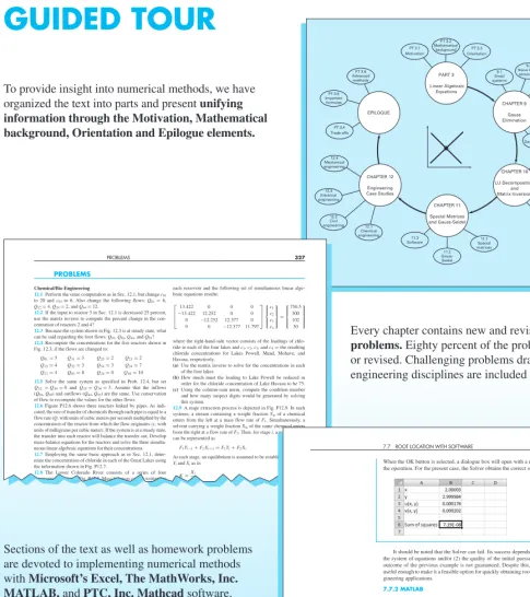
GUIDED TOUR
To provide insight into numerical methods, we have organized the text into parts and present unifying information through the Motivation, Mathematical background, Orientation and Epilogue elements.
Every chapter contains new and revised homework problems.Eighty percent of the problems are new or revised. Challenging problems drawn from all engineering disciplines are included in the text.
Sections of the text as well as homework problems are devoted to implementing numerical methods with Microsoft’s Excel, The MathWorks, Inc. MATLAB,and PTC, Inc. Mathcadsoftware.
PT 3.1 Motivation
PT 3.2 Mathematical
background PT 3.3 Orientation 9.1 Small systems 9.2 Naive Gauss elimination PART 3 Linear Algebraic Equations PT 3.6 Advanced methods EPILOGUE CHAPTER 9 Gauss Elimination PT 3.5 Important formulas PT 3.4 Trade-offs 12.4 Mechanical engineering 12.3 Electrical engineering 12.2 Civil engineering 12.1 Chemical engineering 11.3 Software 11.2 Gauss-Seidel 11.1 Special matrices CHAPTER 10 LU Decomposition and Matrix Inversion CHAPTER 11 Special Matrices and Gauss-Seidel CHAPTER 12 Engineering Case Studies 10.3 System condition 10.2 Matrix inverse 10.1 LU decomposition 9.7 Gauss-Jordan 9.6 Nonlinear systems 9.5 Complex systems 9.4 Remedies 9.3 Pitfalls Chemical/Bio Engineering
12.1Perform the same computation as in Sec. 12.1, but change c01 to 20 and c03to 6. Also change the following flows: Q01=6, Q12=4, Q24=2, and Q44=12.
12.2If the input to reactor 3 in Sec. 12.1 is decreased 25 percent, use the matrix inverse to compute the percent change in the con-centration of reactors 2 and 4?
12.3Because the system shown in Fig. 12.3 is at steady state, what can be said regarding the four flows: Q01, Q03, Q44, and Q55?
12.4Recompute the concentrations for the five reactors shown in Fig. 12.3, if the flows are changed to:
Q01=5 Q31=3 Q25=2 Q23=2 Q15=4 Q55=3 Q54=3 Q34=7 Q12=4 Q03=8 Q24=0 Q44=10
12.5Solve the same system as specified in Prob. 12.4, but set Q12=Q54=0 and Q15=Q34=3. Assume that the inflows (Q01, Q03) and outflows (Q44, Q55) are the same. Use conservation of flow to recompute the values for the other flows.
12.6Figure P12.6 shows three reactors linked by pipes. As indi-cated, the rate of transfer of chemicals through each pipe is equal to a flow rate (Q, with units of cubic meters per second) multiplied by the concentration of the reactor from which the flow originates (c,with units of milligrams per cubic meter). If the system is at a steady state, the transfer into each reactor will balance the transfer out. Develop mass-balance equations for the reactors and solve the three simulta-neous linear algebraic equations for their concentrations.
12.7Employing the same basic approach as in Sec. 12.1, deter-mine the concentration of chloride in each of the Great Lakes using the information shown in Fig. P12.7.
12.8The Lower Colorado River consists of a series of four reservoirs as shown in Fig. P12.8. Mass balances can be written for
each reservoir and the following set of simultaneous linear alge-braic equations results:
PROBLEMS 327 PROBLEMS ⎡ ⎢ ⎢ ⎣
13.422 0 0 0
−13.422 12.252 0 0 0 −12.252 12.377 0 0 0 −12.377 11.797
⎤ ⎥ ⎥ ⎦ ⎧ ⎪ ⎪ ⎨ ⎪ ⎪ ⎩ c1 c2 c3 c4 ⎫ ⎪ ⎪ ⎬ ⎪ ⎪ ⎭ = ⎧ ⎪ ⎪ ⎨ ⎪ ⎪ ⎩
750.5 300 102 30 ⎫ ⎪ ⎪ ⎬ ⎪ ⎪ ⎭ where the right-hand-side vector consists of the loadings of chlo-ride to each of the four lakes and c1, c2, c3, and c4=the resulting chloride concentrations for Lakes Powell, Mead, Mohave, and Havasu, respectively.
(a)Use the matrix inverse to solve for the concentrations in each of the four lakes.
(b)How much must the loading to Lake Powell be reduced in order for the chloride concentration of Lake Havasu to be 75. (c)Using the column-sum norm, compute the condition number and how many suspect digits would be generated by solving this system.
12.9A stage extraction process is depicted in Fig. P12.9. In such systems, a stream containing a weight fraction Yinof a chemical enters from the left at a mass flow rate of F1. Simultaneously, a solvent carrying a weight fraction Xinof the same chemical enters from the right at a flow rate of F2. Thus, for stage i, a mass balance can be represented as
F1Yi−1+F2Xi+1=F1Yi+F2Xi (P12.9a) At each stage, an equilibrium is assumed to be established between Yiand Xias in
K=Xi
Yi
(P12.9b)
7.7 ROOT LOCATION WITH SOFTWARE 193
When the OK button is selected, a dialogue box will open with a report on the success of the operation. For the present case, the Solver obtains the correct solution:
It should be noted that the Solver can fail. Its success depends on (1) the condition of the system of equations and/or (2) the quality of the initial guesses. Thus, the successful outcome of the previous example is not guaranteed. Despite this, we have found Solver useful enough to make it a feasible option for quickly obtaining roots in a wide range of en-gineering applications.
7.7.2 MATLAB
As summarized in Table 7.1, MATLAB software is capable of locating roots of single alge-braic and transcendental equations. It is superb at manipulating and locating the roots of polynomials.
The fzerofunction is designed to locate one root of a single function. A simplified representation of its syntax is
fzero(f,x0,options)
where fis the function you are analyzing, x0is the initial guess, and optionsare the opti-mization parameters (these are changed using the function optimset). If optionsare omitted, default values are employed. Note that one or two guesses can be employed. If two guesses are employed they are assumed to bracket a root The following example
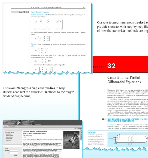
Our text features numerous worked examplesto provide students with step-by-step illustrations of how the numerical methods are implemented.
There are 28 engineering case studiesto help students connect the numerical methods to the major fields of engineering.
Our website contains additional resources for both instructors and students.
913
32
C H A P T E R
32
Case Studies: Partial Differential Equations
The purpose of this chapter is to apply the methods from Part Eight to practical engineer-ing problems. In Sec. 32.1,a parabolic PDE is used to compute the time-variable distribu-tion of a chemical along the longitudinal axes of a rectangular reactor. This example illus-trates how the instability of a solution can be due to the nature of the PDE rather than to properties of the numerical method.
Sections 32.2 and 32.3 involve applications of the Poisson and Laplace equations to civil and electrical engineering problems, respectively. Among other things, this will allow you to see similarities as well as differences between field problems in these areas of engi-neering. In addition, they can be contrasted with the heated-plate problem that has served as our prototype system in this part of the book. Section 32.2deals with the deflection of a square plate, whereas Sec. 32.3is devoted to computing the voltage distribution and charge flux for a two-dimensional surface with a curved edge.
Section 32.4presents a finite-element analysis as applied to a series of springs. This application is closer in spirit to finite-element applications in mechanics and structures than was the temperature field problem used to illustrate the approach in Chap. 31. 32.1 ONE-DIMENSIONAL MASS BALANCE OF A REACTOR
(CHEMICAL/BIO ENGINEERING)
Background. Chemical engineers make extensive use of idealized reactors in their de-sign work. In Secs. 12.1 and 28.1, we focused on single or coupled well-mixed reactors. These are examples of lumped-parameter systems(recall Sec. PT3.1.2).
FIGURE 32.1
An elongated reactor with a single entry and exit point. A mass balance is developed around a finite segment along the tank’s longitudinal axis in order to derive a differential
equation for the concentration. ⌬x
x = 0 x = L
xvii
EXAMPLE 10.4 Matrix Condition Evaluation
Problem Statement. The Hilbert matrix, which is notoriously ill-conditioned, can be represented generally as
⎡ ⎢ ⎢ ⎢ ⎢ ⎢ ⎢ ⎣
1 1/2 1/3 · · · 1/n 1/2 1/3 1/4 · · · 1/(n+1)
. . . .
. . . .
. . . .
1/n 1/(n+1) 1/(n+2) · · · 1/(2n−1) ⎤ ⎥ ⎥ ⎥ ⎥ ⎥ ⎥ ⎦
Use the row-sum norm to estimate the matrix condition number for the 3×3 Hilbert matrix,
[A]=
1 1/2 1/3 1/2 1/3 1/4 1/3 1/4 1/5
Solution. First, the matrix can be normalized so that the maximum element in each row is 1,
[A]=
1 1/2 1/3 1 2/3 1/2 1 3/4 3/5
Summing each of the rows gives 1.833, 2.1667, and 2.35. Thus, the third row has the largest sum and the row-sum norm is
A∞=1+3
4+ 3 5=2.35
The inverse of the scaled matrix can be computed as
[A]−1 =
9 −18 10
−36 96 −60 30 −90 60
xviii
ABOUT THE AUTHORS
Steve Chaprateaches in the Civil and Environmental Engineering Department at Tufts University where he holds the Louis Berger Chair in Computing and Engineering. His other books include Surface Water-Quality Modeling and Applied Numerical Methods with MATLAB.
Dr. Chapra received engineering degrees from Manhattan College and the University of Michigan. Before joining the faculty at Tufts, he worked for the Environmental Protec-tion Agency and the NaProtec-tional Oceanic and Atmospheric AdministraProtec-tion, and taught at Texas A&M University and the University of Colorado. His general research interests focus on surface water-quality modeling and advanced computer applications in environ-mental engineering.
He has received a number of awards for his scholarly contributions, including the 1993 Rudolph Hering Medal (ASCE) and the 1987 Meriam-Wiley Distinguished Author Award (American Society for Engineering Education). He has also been recognized as the out-standing teacher among the engineering faculties at both Texas A&M University (1986 Tenneco Award) and the University of Colorado (1992 Hutchinson Award).
Raymond P. Canaleis an emeritus professor at the University of Michigan. During his over 20-year career at the university, he taught numerous courses in the area of com-puters, numerical methods, and environmental engineering. He also directed extensive research programs in the area of mathematical and computer modeling of aquatic ecosys-tems. He has authored or coauthored several books and has published over 100 scientific papers and reports. He has also designed and developed personal computer software to facilitate engineering education and the solution of engineering problems. He has been given the Meriam-Wiley Distinguished Author Award by the American Society for Engi-neering Education for his books and software and several awards for his technical publications.
3
MODELING, COMPUTERS,
AND ERROR ANALYSIS
PT1.1 MOTIVATION
Numerical methods are techniques by which mathematical problems are formulated so that they can be solved with arithmetic operations. Although there are many kinds of numerical methods, they have one common characteristic: they invariably involve large numbers of tedious arithmetic calculations. It is little wonder that with the development of fast, effi-cient digital computers, the role of numerical methods in engineering problem solving has increased dramatically in recent years.
PT1.1.1 Noncomputer Methods
Beyond providing increased computational firepower, the widespread availability of com-puters (especially personal comcom-puters) and their partnership with numerical methods has had a significant influence on the actual engineering problem-solving process. In the pre-computer era there were generally three different ways in which engineers approached problem solving:
1. Solutions were derived for some problems using analytical, or exact, methods. These solutions were often useful and provided excellent insight into the behavior of some systems. However, analytical solutions can be derived for only a limited class of problems. These include those that can be approximated with linear models and those that have simple geometry and low dimensionality. Consequently, analytical solutions are of limited practical value because most real problems are nonlinear and involve complex shapes and processes.
2. Graphical solutions were used to characterize the behavior of systems. These graphical solutions usually took the form of plots or nomographs. Although graphical techniques can often be used to solve complex problems, the results are not very precise. Furthermore, graphical solutions (without the aid of computers) are extremely tedious and awkward to implement. Finally, graphical techniques are often limited to problems that can be described using three or fewer dimensions.
3. Calculators and slide rules were used to implement numerical methods manually. Although in theory such approaches should be perfectly adequate for solving complex problems, in actuality several difficulties are encountered. Manual calculations are slow and tedious. Furthermore, consistent results are elusive because of simple blunders that arise when numerous manual tasks are performed.
INTERPRETATION
Ease of calculation allows holistic thoughts and intuition to develop; system sensitivity and behavior
can be studied FORMULATION
In-depth exposition of relationship of problem to fundamental
laws
SOLUTION
Easy-to-use computer
method
(b) INTERPRETATION
In-depth analysis limited by time-consuming solution
FORMULATION
Fundamental laws explained
briefly
SOLUTION
Elaborate and often complicated method to make problem tractable
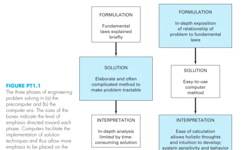
(a) FIGURE PT1.1
The three phases of engineering
problem solving in (a) the
precomputer and (b) the
computer era. The sizes of the boxes indicate the level of emphasis directed toward each phase. Computers facilitate the implementation of solution techniques and thus allow more emphasis to be placed on the creative aspects of problem formulation and interpretation of results.
Today, computers and numerical methods provide an alternative for such compli-cated calculations. Using computer power to obtain solutions directly, you can approach these calculations without recourse to simplifying assumptions or time-intensive tech-niques. Although analytical solutions are still extremely valuable both for problem solv-ing and for providsolv-ing insight, numerical methods represent alternatives that greatly en-large your capabilities to confront and solve problems. As a result, more time is available for the use of your creative skills. Thus, more emphasis can be placed on problem for-mulation and solution interpretation and the incorporation of total system, or “holistic,” awareness (Fig. PT1.1b.)
PT1.1.2 Numerical Methods and Engineering Practice
given us ready access to powerful computational capabilities. There are several additional reasons why you should study numerical methods:
1. Numerical methods are extremely powerful problem-solving tools. They are capable of handling large systems of equations, nonlinearities, and complicated geometries that are not uncommon in engineering practice and that are often impossible to solve analytically. As such, they greatly enhance your problem-solving skills.
2. During your careers, you may often have occasion to use commercially available prepackaged, or “canned,” computer programs that involve numerical methods. The intelligent use of these programs is often predicated on knowledge of the basic theory underlying the methods.
3. Many problems cannot be approached using canned programs. If you are conversant with numerical methods and are adept at computer programming, you can design your own programs to solve problems without having to buy or commission expensive software.
4. Numerical methods are an efficient vehicle for learning to use computers. It is well known that an effective way to learn programming is to actually write computer programs. Because numerical methods are for the most part designed for implementation on computers, they are ideal for this purpose. Further, they are especially well-suited to illustrate the power and the limitations of computers. When you successfully implement numerical methods on a computer and then apply them to solve otherwise intractable problems, you will be provided with a dramatic demonstration of how computers can serve your professional development. At the same time, you will also learn to acknowledge and control the errors of approximation that are part and parcel of large-scale numerical calculations.
5. Numerical methods provide a vehicle for you to reinforce your understanding of mathematics. Because one function of numerical methods is to reduce higher mathematics to basic arithmetic operations, they get at the “nuts and bolts” of some otherwise obscure topics. Enhanced understanding and insight can result from this alternative perspective.
PT1.2 MATHEMATICAL BACKGROUND
Every part in this book requires some mathematical background. Consequently, the intro-ductory material for each part includes a section, such as the one you are reading, on ematical background. Because Part One itself is devoted to background material on math-ematics and computers, this section does not involve a review of a specific mathematical topic. Rather, we take this opportunity to introduce you to the types of mathematical sub-ject areas covered in this book. As summarized in Fig. PT1.2, these are
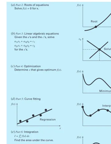
1. Roots of Equations(Fig. PT1.2a). These problems are concerned with the value of a variable or a parameter that satisfies a single nonlinear equation. These problems are especially valuable in engineering design contexts where it is often impossible to explicitly solve design equations for parameters.
2. Systems of Linear Algebraic Equations(Fig. PT1.2b). These problems are similar in spirit to roots of equations in the sense that they are concerned with values that satisfy
f(x)
x Root
x2
x1 Solution
Minimum
f(x)
x Interpolation f(x)
x
f(x)
x Regression
f(x)
I
(a) Part 2: Roots of equations Solve f(x) = 0 for x.
(c) Part 4: Optimization
(b) Part 3: Linear algebraic equations Given the a’s and the c’s, solve a11x1+a12x2=c1
a21x1+a22x2=c2 for the x’s.
Determine x that gives optimum f(x).
(e) Part 6: Integration I=兰abf(x) dx
Find the area under the curve. (d) Part 5: Curve fitting
x
FIGURE PT1.2
equations. However, in contrast to satisfying a single equation, a set of values is sought that simultaneously satisfies a set of linear algebraic equations. Such equations arise in a variety of problem contexts and in all disciplines of engineering. In particular, they originate in the mathematical modeling of large systems of interconnected elements such as structures, electric circuits, and fluid networks. However, they are also encountered in other areas of numerical methods such as curve fitting and differential equations.
3. Optimization (Fig. PT1.2c). These problems involve determining a value or values of an independent variable that correspond to a “best” or optimal value of a function. Thus, as in Fig. PT1.2c, optimization involves identifying maxima and minima. Such problems occur routinely in engineering design contexts. They also arise in a number of other numerical methods. We address both single- and multi-variable unconstrained optimization. We also describe constrained optimization with particular emphasis on linear programming.
4. Curve Fitting(Fig. PT1.2d). You will often have occasion to fit curves to data points. The techniques developed for this purpose can be divided into two general categories: regression and interpolation. Regression is employed where there is a significant degree of error associated with the data. Experimental results are often of this kind. For these situations, the strategy is to derive a single curve that represents the general trend of the data without necessarily matching any individual points. In contrast, interpolation is used where the objective is to determine intermediate values between relatively error-free data points. Such is usually the case for tabulated information. For these situations, the strategy is to fit a curve directly through the data points and use the curve to predict the intermediate values.
5. Integration (Fig. PT1.2e). As depicted, a physical interpretation of numerical integration is the determination of the area under a curve. Integration has many
PT1.2 MATHEMATICAL BACKGROUND 7
y
x
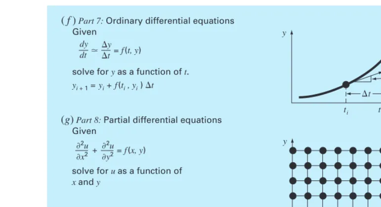
(g) Part 8: Partial differential equations Given
solve for u as a function of x and y
= f(x, y) ⭸2u
⭸x2
⭸2u
⭸y2 +
t Slope = f(ti, yi)
y
⌬t ti ti + 1 (f) Part 7: Ordinary differential equations
Given
solve for y as a function of t. yi + 1=yi+f(ti, yi) ⌬t
⯝ = f(t, y) dy
dt ⌬y ⌬t
applications in engineering practice, ranging from the determination of the centroids of oddly shaped objects to the calculation of total quantities based on sets of discrete measurements. In addition, numerical integration formulas play an important role in the solution of differential equations.
6. Ordinary Differential Equations(Fig. PT1.2f). Ordinary differential equations are of great significance in engineering practice. This is because many physical laws are couched in terms of the rate of change of a quantity rather than the magnitude of the quantity itself. Examples range from population forecasting models (rate of change of population) to the acceleration of a falling body (rate of change of velocity). Two types of problems are addressed: initial-value and boundary-value problems. In addition, the computation of eigenvalues is covered.
7. Partial Differential Equations(Fig. PT1.2g). Partial differential equations are used to characterize engineering systems where the behavior of a physical quantity is couched in terms of its rate of change with respect to two or more independent variables. Examples include the steady-state distribution of temperature on a heated plate (two spatial dimensions) or the time-variable temperature of a heated rod (time and one spatial dimension). Two fundamentally different approaches are employed to solve partial differential equations numerically. In the present text, we will emphasize finite-difference methods that approximate the solution in a pointwise fashion (Fig. PT1.2g). However, we will also present an introduction to finite-element methods, which use a piecewise approach.
PT1.3 ORIENTATION
Some orientation might be helpful before proceeding with our introduction to numerical methods. The following is intended as an overview of the material in Part One. In addition, some objectives have been included to focus your efforts when studying the material.
PT1.3.1 Scope and Preview
Figure PT1.3 is a schematic representation of the material in Part One. We have designed this diagram to provide you with a global overview of this part of the book. We believe that a sense of the “big picture” is critical to developing insight into numerical methods. When reading a text, it is often possible to become lost in technical details. Whenever you feel that you are losing the big picture, refer back to Fig. PT1.3 to reorient yourself. Every part of this book includes a similar figure.
Figure PT1.3 also serves as a brief preview of the material covered in Part One.
Chapter 1is designed to orient you to numerical methods and to provide motivation by demonstrating how these techniques can be used in the engineering modeling process.
PT1.3 ORIENTATION 9 CHAPTER 1 Mathematical Modeling and Engineering Problem Solving PART 1 Modeling, Computers, and Error Analysis CHAPTER 2 Programming and Software CHAPTER 3 Approximations and Round-Off Errors CHAPTER 4 Truncation Errors and the
Taylor Series EPILOGUE 2.7 Languages and libraries 2.6 Mathcad 2.5 MATLAB 2.4 Excel 2.3 Modular programming 2.2 Structured programming 2.1 Packages and programming PT 1.2 Mathematical background PT 1.6 Advanced methods PT 1.5 Important formulas 4.4 Miscellaneous errors 4.3 Total numerical error 4.2 Error propagation 4.1 Taylor series 3.4 Round-off errors 3.1 Significant figures 3.3 Error definitions 3.2 Accuracy and precision PT 1.4 Trade-offs PT 1.3 Orientation PT 1.1 Motivation 1.2 Conservation laws 1.1 A simple model FIGURE PT1.3
PT1.3.2 Goals and Objectives
Study Objectives. Upon completing Part One, you should be adequately prepared to embark on your studies of numerical methods. In general, you should have gained a fun-damental understanding of the importance of computers and the role of approximations and errors in the implementation and development of numerical methods. In addition to these general goals, you should have mastered each of the specific study objectives listed in Table PT1.1.
Computer Objectives. Upon completing Part One, you should have mastered sufficient computer skills to develop your own software for the numerical methods in this text. You should be able to develop well-structured and reliable computer programs on the basis of pseudocode, flowcharts, or other forms of algorithms. You should have developed the ca-pability to document your programs so that they may be effectively employed by users. Finally, in addition to your own programs, you may be using software packages along with this book. Packages like Excel, Mathcad, or The MathWorks, Inc. MATLAB®program are examples of such software. You should become familiar with these packages, so that you will be comfortable using them to solve numerical problems later in the text.
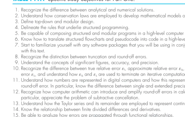
TABLE PT1.1 Specific study objectives for Part One.
1. Recognize the difference between analytical and numerical solutions.
2. Understand how conservation laws are employed to develop mathematical models of physical systems. 3. Define top-down and modular design.
4. Delineate the rules that underlie structured programming.
5. Be capable of composing structured and modular programs in a high-level computer language. 6. Know how to translate structured flowcharts and pseudocode into code in a high-level language. 7. Start to familiarize yourself with any software packages that you will be using in conjunction
with this text.
8. Recognize the distinction between truncation and round-off errors. 9. Understand the concepts of significant figures, accuracy, and precision.
10. Recognize the difference between true relative error εt, approximate relative error εa, and acceptable error εs, and understand how εaand εsare used to terminate an iterative computation.
11. Understand how numbers are represented in digital computers and how this representation induces round-off error. In particular, know the difference between single and extended precision. 12. Recognize how computer arithmetic can introduce and amplify round-off errors in calculations. In
particular, appreciate the problem of subtractive cancellation.
13. Understand how the Taylor series and its remainder are employed to represent continuous functions. 14. Know the relationship between finite divided differences and derivatives.
15. Be able to analyze how errors are propagated through functional relationships. 16. Be familiar with the concepts of stability and condition.
PT1.1 MOTIVATION 11
11
Mathematical Modeling and
Engineering Problem Solving
Knowledge and understanding are prerequisites for the effective implementation of any tool. No matter how impressive your tool chest, you will be hard-pressed to repair a car if you do not understand how it works.
This is particularly true when using computers to solve engineering problems. Al-though they have great potential utility, computers are practically useless without a funda-mental understanding of how engineering systems work.
This understanding is initially gained by empirical means—that is, by observation and experiment. However, while such empirically derived information is essential, it is only half the story. Over years and years of observation and experiment, engineers and scientists have noticed that certain aspects of their empirical studies occur repeatedly. Such general behavior can then be expressed as fundamental laws that essentially embody the cumula-tive wisdom of past experience. Thus, most engineering problem solving employs the two-pronged approach of empiricism and theoretical analysis (Fig. 1.1).
It must be stressed that the two prongs are closely coupled. As new measurements are taken, the generalizations may be modified or new ones developed. Similarly, the general-izations can have a strong influence on the experiments and observations. In particular, generalizations can serve as organizing principles that can be employed to synthesize ob-servations and experimental results into a coherent and comprehensive framework from which conclusions can be drawn. From an engineering problem-solving perspective, such a framework is most useful when it is expressed in the form of a mathematical model.
The primary objective of this chapter is to introduce you to mathematical modeling and its role in engineering problem solving. We will also illustrate how numerical methods figure in the process.
1.1 A SIMPLE MATHEMATICAL MODEL
A mathematical modelcan be broadly defined as a formulation or equation that expresses the essential features of a physical system or process in mathematical terms. In a very gen-eral sense, it can be represented as a functional relationship of the form
Dependent variable = f
independent
variables , parameters,
forcing functions
(1.1)
1
where the dependent variableis a characteristic that usually reflects the behavior or state of the system; the independent variablesare usually dimensions, such as time and space, along which the system’s behavior is being determined; the parametersare reflective of the system’s properties or composition; and the forcing functionsare external influences acting upon the system.
The actual mathematical expression of Eq. (1.1) can range from a simple algebraic re-lationship to large complicated sets of differential equations. For example, on the basis of his observations, Newton formulated his second law of motion, which states that the time rate of change of momentum of a body is equal to the resultant force acting on it. The math-ematical expression, or model, of the second law is the well-known equation
F =ma (1.2)
where F =net force acting on the body (N, or kg m/s2), m
=mass of the object (kg), and
a=its acceleration (m/s2).
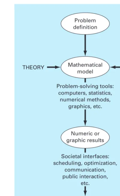
Implementation Numeric or graphic results
Mathematical model Problem definition
THEORY DATA
Problem-solving tools: computers, statistics,
numerical methods, graphics, etc.
Societal interfaces: scheduling, optimization,
communication, public interaction,
etc.
FIGURE 1.1
The second law can be recast in the format of Eq. (1.1) by merely dividing both sides by mto give
a= F
m (1.3)
where a=the dependent variable reflecting the system’s behavior, F=the forcing func-tion, and m=a parameter representing a property of the system. Note that for this simple case there is no independent variable because we are not yet predicting how acceleration varies in time or space.
Equation (1.3) has several characteristics that are typical of mathematical models of the physical world:
1. It describes a natural process or system in mathematical terms.
2. It represents an idealization and simplification of reality. That is, the model ignores negligible details of the natural process and focuses on its essential manifestations. Thus, the second law does not include the effects of relativity that are of minimal im-portance when applied to objects and forces that interact on or about the earth’s surface at velocities and on scales visible to humans.
3. Finally, it yields reproducible results and, consequently, can be used for predictive purposes. For example, if the force on an object and the mass of an object are known, Eq. (1.3) can be used to compute acceleration.
Because of its simple algebraic form, the solution of Eq. (1.2) can be obtained easily. However, other mathematical models of physical phenomena may be much more complex, and either cannot be solved exactly or require more sophisticated mathematical techniques than simple algebra for their solution. To illustrate a more complex model of this kind, Newton’s second law can be used to determine the terminal velocity of a free-falling body near the earth’s surface. Our falling body will be a parachutist (Fig. 1.2). A model for this case can be derived by expressing the acceleration as the time rate of change of the veloc-ity (dv/dt) and substituting it into Eq. (1.3) to yield
dv dt =
F
m (1.4)
where vis velocity (m/s) and tis time (s). Thus, the mass multiplied by the rate of change of the velocity is equal to the net force acting on the body. If the net force is positive, the object will accelerate. If it is negative, the object will decelerate. If the net force is zero, the object’s velocity will remain at a constant level.
Next, we will express the net force in terms of measurable variables and parameters. For a body falling within the vicinity of the earth (Fig. 1.2), the net force is composed of two opposing forces: the downward pull of gravity FDand the upward force of air resistance FU:
F =FD+FU (1.5)
If the downward force is assigned a positive sign, the second law can be used to for-mulate the force due to gravity, as
FD=mg (1.6)
where g=the gravitational constant, or the acceleration due to gravity, which is approxi-mately equal to 9.8 m/s2.
1.1 A SIMPLE MATHEMATICAL MODEL 13
FU
FD
FIGURE 1.2
Schematic diagram of the forces acting on a falling
parachutist. FDis the downward
force due to gravity.FUis the
Air resistance can be formulated in a variety of ways. A simple approach is to assume that it is linearly proportional to velocity1and acts in an upward direction, as in
FU = −cv (1.7)
where c=a proportionality constant called the drag coefficient(kg/s). Thus, the greater the fall velocity, the greater the upward force due to air resistance. The parameter c ac-counts for properties of the falling object, such as shape or surface roughness, that affect air resistance. For the present case, cmight be a function of the type of jumpsuit or the orien-tation used by the parachutist during free-fall.
The net force is the difference between the downward and upward force. Therefore, Eqs. (1.4) through (1.7) can be combined to yield
dv dt =
mg−cv
m (1.8)
or simplifying the right side,
dv dt =g−
c
mv (1.9)
Equation (1.9) is a model that relates the acceleration of a falling object to the forces act-ing on it. It is a differential equationbecause it is written in terms of the differential rate of change (dv/dt) of the variable that we are interested in predicting. However, in contrast to the solution of Newton’s second law in Eq. (1.3), the exact solution of Eq. (1.9) for the ve-locity of the falling parachutist cannot be obtained using simple algebraic manipulation. Rather, more advanced techniques such as those of calculus, must be applied to obtain an exact or analytical solution. For example, if the parachutist is initially at rest (v=0 at
t =0), calculus can be used to solve Eq. (1.9) for
v(t)= gm c
1−e−(c/m)t
(1.10)
Note that Eq. (1.10) is cast in the general form of Eq. (1.1), where v(t)=the depen-dent variable, t =the independent variable, cand m=parameters, and g=the forcing function.
EXAMPLE 1.1 Analytical Solution to the Falling Parachutist Problem
Problem Statement. A parachutist of mass 68.1 kg jumps out of a stationary hot air bal-loon. Use Eq. (1.10) to compute velocity prior to opening the chute. The drag coefficient is equal to 12.5 kg/s.
Solution. Inserting the parameters into Eq. (1.10) yields
v(t)= 9.8(68.1) 12.5
1−e−(12.5/68.1)t
=53.39
1−e−0.18355t
which can be used to compute
1In fact, the relationship is actually nonlinear and might better be represented by a power relationship such as
t,s v,m/s
0 0.00 2 16.40 4 27.77 6 35.64 8 41.10 10 44.87 12 47.49
⬁ 53.39
According to the model, the parachutist accelerates rapidly (Fig. 1.3). A velocity of 44.87 m/s (100.4 mi/h) is attained after 10 s. Note also that after a sufficiently long time, a constant velocity, called the terminal velocity,of 53.39 m/s (119.4 mi/h) is reached. This velocity is constant because, eventually, the force of gravity will be in balance with the air resistance. Thus, the net force is zero and acceleration has ceased.
Equation (1.10) is called an analytical,or exact, solutionbecause it exactly satisfies the original differential equation. Unfortunately, there are many mathematical models that cannot be solved exactly. In many of these cases, the only alternative is to develop a nu-merical solution that approximates the exact solution.
As mentioned previously, numerical methodsare those in which the mathematical problem is reformulated so it can be solved by arithmetic operations. This can be illustrated
1.1 A SIMPLE MATHEMATICAL MODEL 15
0 0 20 40
4 8 12
t,s
v
, m/s
Terminal velocity FIGURE 1.3
for Newton’s second law by realizing that the time rate of change of velocity can be ap-proximated by (Fig. 1.4):
dv
dt
∼
= v
t =
v(ti+1)−v(ti)
ti+1−ti
(1.11)
wherevandt=differences in velocity and time, respectively, computed over finite in-tervals,v(ti)=velocity at an initial timeti,andv(ti+1)=velocity at some later timeti+1.
Note thatdv/dt ∼=v/tis approximate becausetis finite. Remember from calculus that
dv
dt =limt→0
v t
Equation (1.11) represents the reverse process.
Equation (1.11) is called a finite divided differenceapproximation of the derivative at time ti.It can be substituted into Eq. (1.9) to give
v(ti+1)−v(ti)
ti+1−ti
=g− c
mv(ti)
This equation can then be rearranged to yield
v(ti+1)=v(ti)+
g− c
mv(ti)
(ti+1−ti) (1.12)
Notice that the term in brackets is the right-hand side of the differential equation itself [Eq. (1.9)]. That is, it provides a means to compute the rate of change or slope of v.Thus, the differential equation has been transformed into an equation that can be used to deter-mine the velocity algebraically at ti+1using the slope and previous values of vand t.If you
are given an initial value for velocity at some time ti, you can easily compute velocity at a
v(ti +1)
v(ti )
⌬v
True slope dv/dt
Approximate slope
⌬v
⌬t
v(ti +1) –v(ti )
ti +1–ti
=
ti +1
ti t
⌬t
FIGURE 1.4
The use of a finite difference to approximate the first derivative
later time ti+1. This new value of velocity at ti+1 can in turn be employed to extend the
computation to velocity at ti+2and so on. Thus, at any time along the way,
New value=old value+slope×step size
Note that this approach is formally called Euler’s method.
EXAMPLE 1.2 Numerical Solution to the Falling Parachutist Problem
Problem Statement. Perform the same computation as in Example 1.1 but use Eq. (1.12) to compute the velocity. Employ a step size of 2 s for the calculation.
Solution. At the start of the computation (ti =0), the velocity of the parachutist is zero.
Using this information and the parameter values from Example 1.1, Eq. (1.12) can be used to compute velocity at ti+1 =2 s:
v=0+
9.8−12.5
68.1(0) 2=19.60 m/s
For the next interval (from t=2 to 4 s), the computation is repeated, with the result
v=19.60+
9.8−12.5
68.1(19.60) 2=32.00 m/s
The calculation is continued in a similar fashion to obtain additional values:
t,s v,m/s
0 0.00 2 19.60 4 32.00 6 39.85 8 44.82 10 47.97 12 49.96
⬁ 53.39
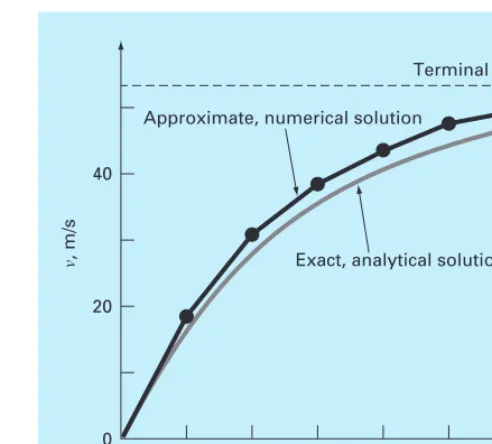
The results are plotted in Fig. 1.5 along with the exact solution. It can be seen that the numerical method captures the essential features of the exact solution. However, because we have employed straight-line segments to approximate a continuously curving function, there is some discrepancy between the two results. One way to minimize such discrepan-cies is to use a smaller step size. For example, applying Eq. (1.12) at l-s intervals results in a smaller error, as the straight-line segments track closer to the true solution. Using hand calculations, the effort associated with using smaller and smaller step sizes would make such numerical solutions impractical. However, with the aid of the computer, large num-bers of calculations can be performed easily. Thus, you can accurately model the velocity of the falling parachutist without having to solve the differential equation exactly.
As in the previous example, a computational price must be paid for a more accurate numerical result. Each halving of the step size to attain more accuracy leads to a doubling
of the number of computations. Thus, we see that there is a trade-off between accuracy and computational effort. Such trade-offs figure prominently in numerical methods and consti-tute an important theme of this book. Consequently, we have devoted the Epilogue of Part One to an introduction to more of these trade-offs.
1.2 CONSERVATION LAWS AND ENGINEERING
Aside from Newton’s second law, there are other major organizing principles in engineer-ing. Among the most important of these are the conservation laws. Although they form the basis for a variety of complicated and powerful mathematical models, the great conserva-tion laws of science and engineering are conceptually easy to understand. They all boil down to
Change=increases−decreases (1.13)
This is precisely the format that we employed when using Newton’s law to develop a force balance for the falling parachutist [Eq. (1.8)].
Although simple, Eq. (1.13) embodies one of the most fundamental ways in which conservation laws are used in engineering—that is, to predict changes with respect to time. We give Eq. (1.13) the special name time-variable(or transient) computation.
Aside from predicting changes, another way in which conservation laws are applied is for cases where change is nonexistent. If change is zero, Eq. (1.13) becomes
Change=0=increases−decreases
or
Increases=decreases (1.14)
0 0 20 40
4 8 12
t,s
v
, m/s
Terminal velocity
Exact, analytical solution Approximate, numerical solution
FIGURE 1.5
Thus, if no change occurs, the increases and decreases must be in balance. This case, which is also given a special name—the steady-statecomputation—has many applications in en-gineering. For example, for steady-state incompressible fluid flow in pipes, the flow into a junction must be balanced by flow going out, as in
Flow in=flow out
For the junction in Fig. 1.6, the balance can be used to compute that the flow out of the fourth pipe must be 60.
For the falling parachutist, steady-state conditions would correspond to the case where the net force was zero, or [Eq. (1.8) with dv/dt=0]
mg=cv (1.15)
Thus, at steady state, the downward and upward forces are in balance, and Eq. (1.15) can be solved for the terminal velocity
v=mg
c
Although Eqs. (1.13) and (1.14) might appear trivially simple, they embody the two fundamental ways that conservation laws are employed in engineering. As such, they will form an important part of our efforts in subsequent chapters to illustrate the connection be-tween numerical methods and engineering. Our primary vehicles for making this connec-tion are the engineering applicaconnec-tions that appear at the end of each part of this book.
Table 1.1 summarizes some of the simple engineering models and associated conserva-tion laws that will form the basis for many of these engineering applicaconserva-tions. Most of the chemical engineering applications will focus on mass balances for reactors. The mass bal-ance is derived from the conservation of mass. It specifies that the change of mass of a chem-ical in the reactor depends on the amount of mass flowing in minus the mass flowing out. Both the civil and mechanical engineering applications will focus on models devel-oped from the conservation of momentum. For civil engineering, force balances are utilized to analyze structures such as the simple truss in Table 1.1. The same principles are employed for the mechanical engineering applications to analyze the transient up-and-down motion or vibrations of an automobile.
1.2 CONSERVATION LAWS AND ENGINEERING 19
Pipe 2 Flow in = 80
Pipe 3 Flow out = 120
Pipe 4 Flow out = ? Pipe 1
Flow in = 100
FIGURE 1.6
TABLE 1.1 Devices and types of balances that are commonly used in the four major areas of engineering. For each case, the conservation law upon which the balance is based is specified.
Structure
Civil engineering Conservation of
momentum Chemical engineering
Field Device Organizing Principle Mathematical Expression
Conservation of mass
Force balance:
Mechanical engineering Conservation of
momentum
Machine Force balance:
Electrical engineering Conservation of charge Current balance:
Conservation of energy Voltage balance: Mass balance:
Reactors Input Output
Over a unit of time period
⌬mass = inputs – outputs
At each node
⌺ horizontal forces (FH) = 0
⌺ vertical forces (FV) = 0
For each node
⌺ current (i) = 0
Around each loop
⌺ emf’s – ⌺ voltage drops for resistors = 0
⌺ – ⌺ iR = 0
–FV
+FV
+FH
–FH
+i2 –i3 +i1
+
–
Circuit
i1R1
i3R3
i2R2
Upward force
Downward force x= 0
PROBLEMS 21
Finally, the electrical engineering applications employ both current and energy bal-ances to model electric circuits. The current balance, which results from the conservation of charge, is similar in spirit to the flow balance depicted in Fig. 1.6. Just as flow must bal-ance at the junction of pipes, electric current must balbal-ance at the junction of electric wires. The energy balance specifies that the changes of voltage around any loop of the circuit must add up to zero. The engineering applications are designed to illustrate how numerical methods are actually employed in the engineering problem-solving process. As such, they will permit us to explore practical issues (Table 1.2) that arise in real-world applications. Making these connections between mathematical techniques such as numerical methods and engineering practice is a critical step in tapping their true potential. Careful examina-tion of the engineering applicaexamina-tions will help you to take this step.
TABLE 1.2 Some practical issues that will be explored in the engineering applications at the end of each part of this book.
1. Nonlinear versus linear.Much of classical engineering depends on linearization to permit analytical solutions. Although this is often appropriate, expanded insight can often be gained if nonlinear problems are examined.
2. Large versus small systems.Without a computer, it is often not feasible to examine systems with over three interacting components. With computers and numerical methods, more realistic multicomponent systems can be examined.
3. Nonideal versus ideal.Idealized laws abound in engineering. Often there are nonidealized alternatives that are more realistic but more computationally demanding. Approximate numerical approaches can facilitate the application of these nonideal relationships.
4. Sensitivity analysis.Because they are so involved, many manual calculations require a great deal of time and effort for successful implementation. This sometimes discourages the analyst from implementing the multiple computations that are necessary to examine how a system responds under different conditions. Such sensitivity analyses are facilitated when numerical methods allow the computer to assume the computational burden.
5. Design.It is often a straightforward proposition to determine the performance of a system as a function of its parameters. It is usually more difficult to solve the inverse problem—that is, determining the parameters when the required performance is specified. Numerical methods and computers often permit this task to be implemented in an efficient manner.
PROBLEMS
1.1 Use calculus to solve Eq. (1.9) for the case where the initial
velocity, v(0)is nonzero.
1.2 Repeat Example 1.2. Compute the velocity to t= 10 s, with a
step size of (a)1 and (b)0.5 s. Can you make any statement
re-garding the errors of the calculation based on the results?
1.3 Rather than the linear relationship of Eq. (1.7), you might
choose to model the upward force on the parachutist as a second-order relationship,
FU = −c′v2
where c′=a second-order drag coefficient (kg/m).
(a) Using calculus, obtain the closed-form solution for the case
where the jumper is initially at rest (v=0 at t=0).
(b) Repeat the numerical calculation in Example 1.2 with the
same initial condition and parameter values. Use a value of 0.225 kg/m for c′.
1.4 For the free-falling parachutist with linear drag, assume a first
jumper is 70 kg and has a drag coefficient of 12 kg/s. If a second jumper has a drag coefficient of 15 kg/s and a mass of 75 kg, how long will it take him to reach the same velocity the fi