Autonomous River Navigation Using the Hamilton–Jacobi Framework for Underactuated Vehicles
Kevin Weekly, Andrew Tinka, Leah Anderson, and Alexandre M. Bayen
Abstract—The feasibility of drifter studies in complex and tidally forced water networks has been greatly expanded by the introduction of motorized floating sensors. This paper presents a method for such motorized sensors to accomplish obstacle avoidance and path selection using the solutions to Hamilton–Jacobi–Bellman–Isaacs (HJBI) equations. The method is then validated experimentally.
Index Terms—Remote sensing, robot control.
I. INTRODUCTION
For several years, the floating sensor network (FSN) project at the University of California at Berkeley (UC Berkeley) [1]–[3] has been deploying floating sensor units, calleddrifters, into various California waterways. The latest generation of such drifters, dubbedGeneration 3[4], has been enhanced by a buoyancy control and dual motor system for autonomous actuation. Each drifter contains aglobal positioning system(GPS) receiver andglobal system for mobile communications cell-phone modem, allowing telemetry readings to be reported to an Internet server in real time. The readings are interpreted as a remote indication of local flow velocity and are integrated with existing forward mathematical models to improve upon flow estimations in real time. Ultimately, it is hoped that this system can be used to populate a map of water conditions to provide interested parties with up-to-date information on tidal conditions or the spread of a contaminant in a region being monitored.
Aquatic drifters, i.e., electromechanical units whose trajectory is in-tended to match the surrounding water, have been developed since the 1950s for oceanographic research. These have been quite successful in the ocean where fixed infrastructure can be impractical to install in the deep sea, and where actuated gliders add dynamic measurement capabilities [5]. Although there has certainly been research into drifters in the river environment [6], [7], drifters have yet to be adopted widely nor used for much more than feasibility studies. River and estuarial environments present extensive obstacles, including underwater veg-etation, channel banks, and man-made structures, that are essentially absent from the ocean environment. Applying drifter technology to inland environments, therefore, requires addressing the obstacle chal-lenge directly. Typically, passive drifters are supervised by personnel in boats, who retrieve the drifters when they get snagged on obsta-cles. Adding limited propulsion and autonomous obstacle avoidance
Manuscript received September 18, 2013; revised March 15, 2014; accepted May 20, 2014. Date of publication June 18, 2014; date of current version September 30, 2014. This paper was recommended for publication by Associate Editor K. Kyriakopoulos and Editor G. Oriolo upon evaluation of this reviewer’s comments.
K. Weekly, A. Tinka, and A. M. Bayen are with the Department of Elec-trical Engineering and Computer Sciences, University of California, Berke-ley, CA 94720 USA (e-mail: [email protected]; [email protected]; [email protected]).
L. Anderson is with the Department of Civil and Environmental En-gineering, University of California, Berkeley, CA 94720 USA (e-mail: [email protected]).
Color versions of one or more of the figures in this paper are available online at http://ieeexplore.ieee.org.
Digital Object Identifier 10.1109/TRO.2014.2327288
to the floating drifters is an approach that sets the FSN project apart from other river drifter research. The FSN project is the first to de-sign motorized drifters to be low-cost and manufacturable, allowing us to produce a fleet of 40 and demonstrate their success in a field experiment.
In this paper, we address the problem of obstacle avoidance and path selection in an environmental setting. The obstacle avoidance task is the ability of the drifters to avoid becoming stuck on haz-ards. To comprehensively understand water conditions, it is also nec-essary for a drifter fleet to distribute itself among multiple paths throughout the water system, which we refer to as thepath-selection task.
Controlling in the presence of obstacles is linked to path plan-ning problems [8]–[10], which sometimes rely on the Hamilton– Jacobi and optimal control theory, such as [11]. Recently, Lollaet al. [12] demonstrated in simulation a path planning algorithm using nearly the same theory as described in [13] and this paper. Two fea-tures of our problem distinguish it from the traditional path planning problem.
1) The drifter is an underactuated system. That is, the unit is in the presence of a river current which is more powerful than the propul-sion of the unit. Thus, a successful algorithm must account for the river current and act preemptively to avoid being pushed into an obstacle.
2) Our goal is not to reach a single target waypoint; rather, the goal of the drifter is to not run into obstacles.
Several approaches can be used to solve these types of problems. Viability-based approaches compute regions of the state space such as “all points guaranteed to be safe” [14], [15]. Another approach is to use the level and sublevel sets of solutions toHamilton–Jacobi– Bellman–Isaacs (HJBI)equations [16]–[20]. We chose to use the HJBI framework, which can be used to compute the same sets, in order to use an existing mathematical toolbox [21] to solve these equations numerically.
We show that the solution to an HJBI equation can be used to construct aminimum-time-to-reach(MTTR) function to a given target region. Two such MTTR functions, i.e.,Vc e nte r andVsh o re, are used
to determine the transitions of the ON–OFFcontroller. With the proper MTTR function, it is also possible to find the optimal control policy, i.e., the direction in which to travel in order to reach a target the quickest. It is well known that because the HJBI equation is derived by application of dynamic programming(DP) techniques [18], synthesizing these MTTR functions suffers the same curse of dimensionality as other DP methods [22]. Fortunately, for low-dimensional systems, such as described in this paper, the problem is tractable.
The drifter unit’s measured velocity matches the local water velocity only while the drifter isnotunder actuation. Thus, we seek to maximize the amount of time the motors are turned completely OFF. ON–OFF control is, therefore, a natural choice, since it specifies using maximum actuation or none at all. It then remains to determine the on-state policy and thresholds of the ON–OFFcontroller.
We presented and demonstrated via field testing a practical solution to the obstacle avoidance challenge in [13]. This paper extends this by showing that an intuitive change to the inputs of the algorithm accom-plishes the path-selection task. We also demonstrate the path-selection task with a field test at a fork in the Sacramento river. We also pro-vide a more detailed description of the platform. The rest of this paper is organized as follows. Section II discusses the method behind the obstacle avoidance and path planning algorithms. Section III provides practical implementation details and simulation results. Section IV presents results from our field operational tests, and finally, we con-clude this paper in Section V.
II. HAMILTON–JACOBI–BELLMAN–ISAACS-BASED OPTIMALCONTROL
A. Model and Problem Statement
We model the system dynamics of a single drifter as a 2-D single integrator:
˙
x=f(x, a, b) =w(x) +a(t) +b(t) (1)
a(t)2 ≤¯a
b(t)2 ≤¯b
wherex∈R2 is a 2-D state vector representing the position of the drifter in meters,a(t)is thecontrol input, andb(t)is thedisturbance input. Note the absence of a yaw state variable, which is intentionally omitted to reduce the computational burden. We believe the term to be largely irrelevant for longer time scales as the vehicle is highly maneuverable around its vertical axis, owing to the differential drive configuration.
An estimate of the river current,w(x), is given by a forward simula-tion of the regionwithoutintegration of drifter-collected data. Note that although the purpose of the FSN project as a whole is to provide more accurate estimates of the river currents using the drifters, nevertheless, a less-accurate simulation can be used for the purposes of control. As the river current estimates improve by integrating the drifter-collected data, then the control will also benefit for future experiments by having a more accurately specifiedw(x).
We also define the following sets of functions and parameters:¯aand ¯b:
A{a(·) :a(t)2 ≤¯a∀t} B%b
(·) :b(t)2 ≤¯b∀t &
and parameterize the trajectory of the system in terms of time, initial condition, and thea(·)andb(·)inputs
x=x(t;x0, a(·), b(·)).
With these functions, we will set up adifferential game [17], [23] in which the inputs a(·) andb(·) work against each other to either satisfy or attempt to violate a safety condition, respectively. As we will see later,b(·)will always act in the opposite direction ofa(·)with magnitude¯b. Therefore, in this case, running this differential game with input constraints(¯a,¯b)is equivalent to running a single-player game with input constraints(¯a−¯b,0), although this is not true for general differential games [23].
To set up this game, we are given a set of undesirable positions,
Tsh o re ⊂R2 corresponding to collisions with obstacles. Conversely,
the complement of this set, i.e.,STC
sh o re, gives the positions for
which the system issafe.
Our goal is to find a control inputa(·)such that
∀t >0, ∀x0 ∈ S,∀b(·)∈B, x(t;x0, a(·), b(·))∈ S. (2)
Ideally,a(·)also minimizes the time of actuation ta c t=
However, the proposed algorithm does not necessarily produce an op-timala(·)in this respect.
B. Mathematical Solutions
In this section, we describe the meaning of an MTTR in the context of HJBI equations. In the next section, we describe several MTTR functions used in an algorithm to satisfy (2). We begin with atarget set,T ⊂Rn, giving a set of states we are trying to reach. Consider the
construction of astatic cost function,V(x0):
V(x0) =
Rni)→Ris a Lagrangian cost functional associ-ating a cost for the system to be in a certain state and taking a certain action.
Thus, the interpretation of (4) is that it designates the first time the trajectoryx(·;a(·), b(·))entersT.
Suppose we takel(·,·,·)≡1, representing a constant accrual of cost until the target set is reached. Substituting into (3)
V(x0) = inf
wherea⋆(·)is called theoptimal controlfor this particular cost function
as it minimizes the accrued cost, andb⋆(·)is theworst-casedisturbance.
In this case, (6) simply gives the minimum time to reach the target setT fromx0; therefore, we callV an MTTR function for this system.
Note that V(x0) = +∞ in the case in which the target set is not
reachable from the initial conditionx0.
We are interested in finding the optimal control, or disturbance, which satisfies (7) and achieves a minimum-time trajectory to, or from,
T. Both can be computed explicitly as a function of the gradient of the MTTR function by the following relations:
a⋆(x) =−¯a ∇V(x)
∇V(x)2
, b⋆(x) = ¯b ∇V(x)
∇V(x)2
. (8)
In general,V is difficult to compute especially for systems such as (1) which have an arbitrary forcing term,w, and an arbitrary target set,T. We elect to extend the technique found in [21] for finding the MTTR function of a holonomic system: Atime-dependent HJBIequation, for which there are known methods to solve [24], is constructed as follows:
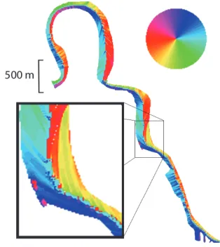
Fig. 1. Example flow field estimate from REALM forward simulation model of the Walnut Grove experimental region near the river split (see Fig. 4).
noting that althoughφ is, by definition, discontinuous att= 0, by using the Lax–Friedrichs numerical method, this discontinuity is be dissipated and the solution is stable [18], [21].
As shown in [17],T can be reached inhtime or less from the set of points
G(h) ={x:φ(x, h)≤0}.
The frontier of this set of points as it evolves through time is also the set of points from whichT can be reached in exactlyhtime. The set is related toV by
∂G(h) ={x:φ(x, h) = 0}.
Consider a contour {x:V(x) =h} of the MTTR function, de-scribing a set of points reachable in exactly h time units. Comparing this contour with∂G(h), we find that, for a givenx,V(x) is given by the first temporal zero crossing ofφ(x, t). If such a zero crossing does not exist, this means the system cannot navigate from xtoT; therefore,V(x) = +∞. This zero crossing can be calculated numerically as in [21].
III. IMPLEMENTATION
A. Flow Field Modeling
We use flow field estimates from REALM, which is a forward nu-merical model of the Sacramento–San Joaquin Delta [25], for the values ofw(x)required for computation. An example of a flow field produced from this simulation is shown in Fig. 1. Due to the tidal nature of the flows in the area, multiple flow field estimates are taken, corresponding to different times of day. The on-board controller will automatically cycle through the policies throughout the course of the day to account for varying water currents.
B. Computation of Control Feedback
The on-board controller requires three 2-D arrays to be computed offline and loaded before the experiment:
1) The MTTR function toward the shore of the river is designated Vsh o re. TheVsh o reMTTR satisfies (5), where¯a >0is the maximum
current speed which could push the drifter to the shore, no other force disturbs the drift (¯b= 0), and T =Tsh o re, the left binary
image from Fig. 2. The function, therefore, describes how much time the vehicle would move, pushed at speed¯a, before crashing on the shore.
2) The MTTR function toward the center of the river is designated as Vc e nte r. This function also satisfies (5), where¯a >0is the maximal
propulsion of the drifter,¯bis the maximal disturbance, andT = Tc e nte ris the right binary image from Fig. 2.
Fig. 2. (Left)Tsh o re, the constraint set which we want the drifter to avoid.
(Right)Tc e nte r, target set which the drifter needs to reach after touching the
dangerous set.
Fig. 3. Optimal bearing to center of the river,∠⋆(x). A particularly complex
region is zoomed in.
3) The optimal bearing toward the center of the river, which is denoted by ∠⋆(x), and plotted by Fig. 3, is the angle component of the optimal control given in (8), whereV in this relation isVc e nte r.
These three arrays are combined into apolicy filewhich is loaded onto the drifter prior to the experiment. If we repeat this process for different values ofworT, we could generate several such policy files. The drifter is able to select which policy file is used in the on-board controller. For example, the on-board controller could automatically change the policy file over the course of the day to account for periodic tidal flows.
C. Path Selection
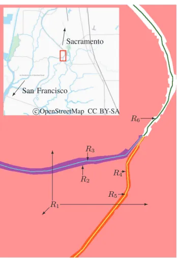
To accomplish path selection, we calculated two policy files for the region shown in Fig. 4, which also illustrates the sets{R1, . . . , R6}.
The first policy file is loaded on drifters which should go down the west path and is generated with the inputs
Tsh o re ←R1∪R4 ∪R5
Tc e nte r ←R6 ∪R3
and the second policy file is loaded on drifters which should go down the east path and generated with the inputs
Tsh o re ←R1∪R2 ∪R3
Fig. 4. Source files for lane-splitting algorithm superimposed and color-coded and map showing geographic location. Each color represents a set of points and is labeled for reference.
Fig. 5. On-board controller hybrid automaton diagram.
For each case, we are treating the unselected path as an obstacle and the selected path as the only viable option for the drifter to be directed.
D. On-Board Controller
Within this framework, our on-board ON–OFFcontrol system can be encoded by a hybrid automatonH= (Q, X, R, f,Σ,U)[26], [27]. Qis the set of the two modes{qdrift, qactuate}, which the drifter
alter-nates between during its mission. X is the domain of the drifter’s location R2. Σ is the set of discrete events which can trigger a
transition between modes, and in our case, Σ ={x∈ L, x∈ D}. R: (Q,Σ, X)→(Q, X)is the transition function, encoded by Fig. 5. fq:X→X are the dynamics experienced while in each mode, also
shown in Fig. 5. Finally,U is the set of inputs afforded to the drifter
U=A={a(·) :∀ta(t)2 ≤a¯}.
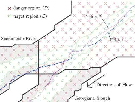
Thetarget regionLanddanger regionDare defined as follows:
L {x:Vc e nte r(x)≤8s} ∩ C
D{x:Vsh o re(x)≤300s} \ L.
Thus, when the position of the drifter is in danger, i.e.,x∈ D, the controller turns on the motors and seeks the optimal trajectory back to safety. When the drifter reaches safety, i.e.,x∈ L, the controller turns the motors OFF and resumes passive drifting. Throughout the experiment, we record the state of the controller alongside the GPS measurements in order to later discard measurements taken while the
Fig. 6. Drifter GPS trajectory during northward tidal flow. The red line is a contour ofVsh o reand denotes the edge of the danger region. The green line is
a contour ofVc e nte rand defines the target region. Along the drifter trajectory,
dotted lines indicate unactuated motion. See Fig. 1 for the simulated flow in the region during the experiment.
drifter was actuating. This ensures that only data corresponding to passive drifting are used for later estimation (assuming, as in our case, that the estimator does not need a continuous trajectory but only point velocity measurements).
IV. FIELDOPERATIONALTESTS
A. Obstacle Avoidance
A field operational test was carried out targeting the Sacramento– San Joaquin River Delta in California (approximately Latitude 38.03 N, Longitude 121.58 W). The controller described in Section III was tested for approximately 5 h in the river. Two boat teams were responsible for monitoring the drifters and retrieving trapped units if necessary. Retrieved drifters were placed back in the river at safe locations to continue their mission. One goal of the experiment was to determine if the controller presented in this paper effectively prevented the drifters from heading into dangerous areas, therefore reducing the number of necessary retrievals.
Fig. 6 shows data from the field deployment that was gathered by one of the units. The trajectory of the unit has been reconstructed from GPS positions recorded on-board and plotted by the solid magenta and dotted blue lines, where the magenta lines and dotted blue lines indicate when the controller was inqactuateandqdrift, respectively.
This result demonstrates behavior similar to that predicted by pre-viously simulated results. During deployment, an easterly wind threat-ened to beach the drifters. Here, this drifter floats north with the river current, but is also being pushed toward the eastern shoreline. Upon crossing theVsh o rethreshold (red contour), it begins to maneuver back
to safety. Once it reaches theVc e nte rthreshold (green contour), it
Fig. 7. GPS trajectories of two drifters performing the path-selection algo-rithm during a field test in Walnut Grove, CA. One of the drifters, shown by the blue trace, is tasked with proceeding down the Sacramento River, while the other drifter, in magenta, is tasked with proceeding down the Georgiana Slough. Along the trajectory, the faded segments indicate passive motion where the motors are OFF.
appears to be sufficient for preventing collisions with the shoreline, but more advanced obstacle avoidance has yet to be proven in the field.
B. Path Selection
In our second experiment, we operated at an interesting fork in the Sacramento river near Walnut Grove, CA, USA (approximately Latitude 38.24 N, Longitude 121.52 W; see Fig. 4). Here, the Georgiana Slough meets the Sacramento river and diverts some quantity of water from it to be used in the delta. The large majority of the water, however, continues down the Sacramento river, taking any nonactuated drifters with it. Hence, our actuated drifters are needed to ensure some part of the fleet ends up traveling down the Georgiana Slough to measure that environment.
The primary goal of this experiment was to divert 10 out of 30 actuated drifters down the Georgiana slough, with the remaining 20 actively remaining in the Sacramento. By designing the proper obstacle map,Tsh o re, we formed two parallel lanes for the drifters to split and
stay within, before the actual split happened. This caused the group of drifters to clearly split into two groups and allows us to retrieve any malfunctioning units before they are in danger. In practice, the algorithm does not require that these lanes are drawn, only that an obstacle be drawn across unselected paths.
Fig. 7 shows a plot of the trajectories of two drifters, one from each group. The data represent a GPS location taken every 2 s by each drifter and passed through a two-element moving average filter to remove sensor noise from the GPS system. Note that, unlike Fig. 6, the drifters clearly enter the danger region; however, this does not indicate a failure to satisfy (2), since the drifter remained withinS. The figure demonstrates that the drifters have successfully actuated in a manner placing them in the correct lane and simultaneously avoiding obstacles.
V. CONCLUSION
In this paper, we have described a successful technique for con-trolling our autonomous floating sensor platforms so that they avoid obstacles and the shoreline during a mission. We showed the efficacy of the algorithm for the scenarios in which the unit must actively avoid
running against the bank of a river and in which the unit must drive itself down a particular fork of the river. We are the first to demon-strate using the solutions of HJBI equations for active duty field work. We also seek to reduce the computational burden of the technique and move toward an online integrated solution.
ACKNOWLEDGMENT
The authors would like to thank I. Mitchell for his level set toolbox and advice on HJBI theory. They would also like to thank Q. Wu, P. Schwartz, and E. Ateljevich for their work with the REALM code.
REFERENCES
[1] (2010). Floating sensor network [Online]. Available: http://float. berkeley.edu/
[2] A. Tinka, I. Strub, Q. Wu, and A. Bayen, “Quadratic programming based data assimilation with passive drifting sensors for shallow water flows,” inProc. 48th IEEE Conf. Decision Control, 2009, pp. 7614–7620. [3] O. Tossavainen, J. Percelay, A. Tinka, Q. Wu, and A. Bayen, “Ensemble
Kalman filter based state estimation in 2D shallow water equations using lagrangian sensing and state augmentation,” inProc. 47th IEEE Conf. Decision Control, 2008, pp. 1783–1790.
[4] A. Tinka, M. Rafiee, and A. M. Bayen, “Floating sensor networks for river studies,”IEEE Syst. J., vol. 7, no. 1, pp. 36–49, Mar. 2013.
[5] R. N. Smith, M. Schwager, S. L. Smith, B. H. Jones, D. Rus, and G. S. Sukhatme, “Persistent ocean monitoring with underwater gliders: Adapting sampling resolution,”J. Field Robot., vol. 28, no. 5, pp. 714– 741, 2011.
[6] J. C. Perez, J. Bonner, F. J. Kelly, and C. Fuller, “Development of a cheap, GPS-based, radio-tracked, surface drifter for closed shallow-water bays,” inProc. IEEE/OES 7th Work. Conf. Current Meas. Technol., Mar. 2003, pp. 66–69.
[7] J. Austin and S. Atkinson, “The design and testing of small, low-cost GPS-tracked surface drifters,”Estuaries, vol. 27, no. 6, pp. 1026–1029, Dec. 2004.
[8] F. Zhang, D. M. Fratantoni, D. A. Paley, J. M. Lund, and N. E. Leonard, “Control of coordinated patterns for ocean sampling,”Int. J. Control, vol. 80, no. 7, pp. 1186–1199, 2007.
[9] J. Latombe,Robot Motion Planning. New York, NY, USA: Springer-Verlag, 1990.
[10] S. LaValle,Planning Algorithms. Cambridge, U.K.: Cambridge Univ. Press, 2006.
[11] S. Sundar and Z. Shiller, “Optimal obstacle avoidance based on the Hamilton-Jacobi-Bellman equation,”IEEE Trans. Robot. Autom., vol. 13, no. 2, pp. 305–310, Apr. 1997.
[12] T. Lolla, M. Ueckermann, K. Yigit, P. J. Haley, and P. F. Lermusiaux, “Path planning in time dependent flow fields using level set methods,” in Proc. Int. Conf. Robot. Autom., 2012, pp. 166–173.
[13] K. Weekly, L. Anderson, A. Tinka, and A. Bayen, “Autonomous river nav-igation using the Hamilton-Jacobi framework for underactuated vehicles,” inProc. Int. Conf. Robot. Autom., 2011, pp. 828–833.
[14] A. Tinka, S. Diemer, L. Madureira, E. Marques, J. Sousa, R. Martins, J. Pinto, J. Silva, A. Sousa, P. Saint-Pierre, and A. Bayen, “Viability-based computation of spatially constrained minimum time trajectories for an autonomous underwater vehicle: Implementation and experiments,” in Proc. Amer. Control Conf., Jun. 2009, pp. 3603–3610.
[15] P. Cardaliaguet, M. Quincampoix, and P. Saint-Pierre, “Set-valued nu-merical analysis for optimal control and differential games,”Stochastic Differential Games, Theory Numerical Methods, vol. 4, pp. 177–247, 1999.
[16] A. Bayen, I. Mitchell, S. Santhanam, and C. Tomlin, “A differential game formulation of alert levels in ETMS data for high altitude traffic,” inProc. AIAA Guidance, Navigation, Control Conf., Aug. 2003, pp. 1–11. DOI: 10.2514/6.2003-5341
[17] I. Mitchell, A. Bayen, and C. Tomlin, “A time-dependent Hamilton-Jacobi formulation of reachable sets for continuous dynamic games,”IEEE Trans. Autom. Control, vol. 50, no. 7, pp. 947–957, Jul. 2005.
[19] J. Sethian,Level Set Methods and Fast Marching Methods: Evolving In-terfaces in Computational Geometry, Fluid Mechanics, Computer Vision, and Materials Science. Cambridge, U.K.: Cambridge Univ. Press, 1999. [20] S. Osher and R. Fedkiw,Level Set Methods and Dynamic Implicit Surfaces,
vol. 153. New York, NY, USA: Springer-Verlag, 2003.
[21] I. Mitchell, “A toolbox of level set methods,” Dept. Comput. Sci., Univ. British Columbia, Vancouver, BC, Canada, Tech. Rep. TR-2007-11, 2007, vol. 11.
[22] R. Bellman,Dynamic Programming. Princeton, NJ, USA: Princeton Univ. Press, 1957.
[23] R. Isaacs,Differential Games: A Mathematical Theory With Applications to Warfare and Pursuit, Control and Optimization. Hoboken, NJ, USA: Wiley, 1965.
[24] S. Osher, “A level set formulation for the solution of the Dirichlet problem for Hamilton–Jacobi equations,”SIAM J. Math. Anal., vol. 24, pp. 1145– 1152, 1993.
[25] E. Ateljevich, P. Colella, D. Graves, T. Ligocki, J. Percelay, P. Schwartz, and Q. Shu, “CFD modeling in the San Francisco bay and delta,” in Proc. 4th SIAM Conf. Math. Ind., 2009, pp. 99–107. DOI: 10.1137/1.9781611973303.12.
[26] J. Lygeros, C. Tomlin, and S. Sastry, “Controllers for reachability spec-ifications for hybrid systems,”Automatica-Oxford, vol. 35, pp. 349–370, 1999.
[27] C. Cassandras and S. Lafortune,Introduction to Discrete Event Systems, vol. 11. Norwell, MA, USA: Kluwer, 1999.
Foot Placement in the Simplest Slope Walker Reveals a Wide Range of Walking Solutions
Pranav A. Bhounsule
Abstract—We show that the simplest slope walker can walk over wide combinations of step lengths and step velocities at a given ramp slope by proper choice of foot placement. We are able to find walking solutions up to slope of 15.42◦, beyond which, the ground reaction force on the stance leg goes to zero, implying a flight phase. We also show that the simplest walker can walk at human-sized step length and step velocity at a slope of 6.62◦. The central idea behind control using foot placement is to balance the potential energy gained during descent with the energy lost during collision at foot-strike. Finally, we give some suggestions on how the ideas from foot placement control and energy balance can be extended to realize walking motions on practical legged systems.
Index Terms—Compass gait, foot placement, passive dynamic walking, Poincar´e map, simplest walker.
I. INTRODUCTION
There is a class of robots, called passive dynamic walkers, that can walk down shallow inclines with no control or energy input. Passive
Manuscript received September 9, 2013; revised February 27, 2014; accepted May 27, 2014. Date of publication June 23, 2014; date of current version September 30, 2014. This paper was recommended for publication by Associate Editor P. Soueres and Editor A. Kheddar upon evaluation of this reviewer’s comments.
The author is with the Disney Research Pittsburgh, Pittsburgh, PA 15213 USA, and also with the Department of Mechanical Engineering, Uni-versity of Texas San Antonio, San Antonio, TX 78249 USA (e-mail: [email protected]).
Color versions of one or more of the figures in this paper are available online at http://ieeexplore.ieee.org.
Digital Object Identifier 10.1109/TRO.2014.2328796
dynamic walkers were first demonstrated in experiment by McGeer [1]. Furthermore, he used tools in dynamical systems, namely, Poincar´e return map to search for walking gaits and eigenvalues of the linearized return map to explain stability of the walking motions.
McGeer found that the robot morphology like mass, inertia, leg length, foot radius, and the ramp slope influences the dynamics of the walking gait. A better insight into the mechanics of passive dy-namic walkers might be achieved by reducing the parameter space. In this spirit, Garcia et al.[2] did an extreme simplification to the passive dynamic walking model analyzed by McGeer. They put a point mass at the hip and infinitesimal point mass at each foot of the straight leg walker. After nondimensionalizing the equations of motion, they demonstrated that the model has only one free parameter: the ramp slope.
The model analyzed by Garciaet al., called the simplest walker, demonstrates two families of period-one walking solutions (a walking motion that repeats itself every step): a stable solution and an unstable solution. There is one stable period-one solution for each slope in the range 0–0.87◦. As the slope is increased beyond 0.87◦, higher period walking emerges, ultimately leading to chaotic walking. There are no stable passive walking solutions for the simplest walker beyond a slope of 1.1◦. On the other hand, there is one unstable period-one solution for each slope in the range 0–15.42◦. Beyond 15.42◦, there are no walking solutions because the ground reaction force on the stance leg goes to zero.
In this paper, we explore the range of walking solutions for the hip-actuated simplest walker. In particular, we use the hip actuator to do accurate foot placement. Using foot placement for control of legged systems is not new. Prattet al.[3] defined the capture point as the location where the robot needs to place its foot to come to a complete stop when pushed. They computed the capture point based on the zero of the orbital energy of the robot idealized as a linear-inverted pendulum with smooth support transfer.
Wightet al.[4] introduced the concept of foot placement estimator, which is identical to the capture point concept. However, unlike Pratt et al., they used the inverted pendulum model with collisional support transfer which is similar to the model used here. We will do analysis similar to that of Prattet al.and Wightet al.to compute the feasible walking solutions for the simplest slope walker [2].
In this paper, by means of theoretical calculations, we demonstrate that: 1) By controlling foot placement in the simplest walker, and a suitable choice of slope, wide combinations of speeds and step lengths are possible. 2) A feed-forward control law that achieves a particular foot placement strategy can be numerically computed. 3) Walking at average human speed and stride length is possible by appropriate choice of slope.
II. BIPEDMODEL
A. Model Description
Fig. 1(a) shows a cartoon of the simplest walker. The model has a massMat the hip and point massmat each of the feet. Each leg has lengthℓ, gravitygpoints downward, and the ramp slope isγ. The leg in contact with the ramp is called the stance leg, while the other leg is called the swing leg. The angle made by the stance leg with the normal to the ramp isθ, and the angle made by the swing leg with the stance leg isφ. The hip torque isU. Fig. 1(b) describes a typical step of the simplest walker. The walker starts in (i), the state in which the front leg is the stance leg and the trailing leg is the swing leg. The walker moves from (ii) to (v) as shown. We ignore foot scuffing. Finally, in (vi), the swing leg collides with the ground and becomes the new stance leg. At