Electric Sensor-Based Control of Underwater
Robot Groups
Christine Chevallereau, Member, IEEE, Mohammed-R´edha Benachenhou, Vincent Lebastard, Member, IEEE,
and Fr´ed´eric Boyer
Abstract—Some fish species use electric sense to navigate effi-ciently in the turbid waters of confined spaces. This paper presents a first attempt to use this sense to control a group of nonholo-nomic rigid underwater vehicles navigating in a cooperative way. A leader whose motion is unknown to the others serves as an active agent for its passive neighbor, which perceives the leader’s elec-tric field via current measurements and moves in order to follow a trajectory relative to it. Then, this passive agent, becomes in its turn the leader for the next agent and so on. Sufficient conditions of convergence of the control law are derived for electric current servoing. This is achieved without the explicit knowledge of the location of the agents. Some limits on the possible motion of the leader along with the importance of the choice of controlled out-puts are demonstrated. Switching between different group config-urations by following a virtual agent is also described. Simulation and experimental results illustrate the theoretical study.
Index Terms—Biologically inspired robots, electric sense, marine robotics, nonholonomic agent, visual servoing.
I. INTRODUCTION
E
LECTRIC sense is a mode of perception used by sharks, rays [1], and several hundreds of fish species of the Gym-notidandMormyridfamilies, who live in the tropical forests of Africa and South America. While sharks and rays pas-sively sense the electric fields generated in their surroundings, mormyrids and gymnotids have developed an active version of this sense by generating their own electric field called a ”basal field” or ”carrier.” While in the gymnotid fish, the carrier has a sine-wave nature, mormyrid fish produce a pulsed dipolar elec-tric field by polarizing on short durations with a specific organ called the electric organ discharge (EOD) located just anterior to the tail with respect to the rest of the body. In all cases, the distortions of this basal field by the surrounding objects are measured by a dense distribution of electroreceptors distributed over the fish’s skin. By processing these measurements, the fishManuscript received July 1, 2013; accepted December 17, 2013. Date of pub-lication January 13, 2014; date of current version June 3, 2014. This paper was recommended for publication by Associate Editor I. H. Suh and Editor B. J. Nelson upon evaluation of the reviewers’ comments. This work was supported by the ANGELS project funded by the European Commission, Information So-ciety and Media, Future and Emerging Technologies under Contract 231845.
The authors are with the Centre national de la recherche scientifique, Ecole des Mines de Nantes, Institut de Recherche en Communication et Cybern´etique de Nantes, Nantes 44321, France (e-mail: Christine.Chevallereau@irccyn. ec-nantes.fr; [email protected]; Vincent. [email protected]; [email protected]).
Color versions of one or more of the figures in this paper are available online at http://ieeexplore.ieee.org.
Digital Object Identifier 10.1109/TRO.2013.2295890
perceive their environment efficiently and can easily navigate in the turbid waters of tropical forests, which are their ecologi-cal niche. Named electrolocation, this sensorial ability has high potential interest for underwater robotics applications such as deep-sea exploration, rescue missions under catastrophic con-ditions or navigation in muddy waters, i.e., under concon-ditions where neither vision nor sonar can work. Based on these obser-vations, roboticists have recently proposed the first bioinspired electric field sensors with the aim of equipping a new gener-ation of underwater vehicles (UVs) able to navigate in turbid waters and confined environments [2]–[5]. In [4], the sensor is an insulating mobile body on the boundaries of which are fixed an arbitrary number of electrodes. A voltage generator imposes a potential on one of these electrodes (located in the tail), with respect to all the others (which are set to a common ground). Once immersed in a conductive fluid, this device produces a nearby dipolar electric field, and by Coulomb’s law, a contin-uous network of closed current lines linking the tail electrode (emitter) to all the others (receivers) across which the currents are measured. In this case, the sensor is said to work in active mode, since it produces the carrier whose modulations by the environment, contain the measured information.
Electric fish also use a passive version of the electric sense in which the fields are not generated by themselves but by some exogenous sources [6]. These exogenous fields can be produced by prey or other nearby electric fish, which is a very usual case, since these fish swim mostly in small social groups of a few individuals [7]. Biological experiments [8]–[12] have re-vealed that active electric fish use specific strategies to organize their collective electric activity. In particular, in order to avoid jamming and overlapping between individual electric pulses, several species of mormyrid order the electric activity of each member of a group in a fixed sequence of individual pulses separated by “silent periods.” On the other hand, the wave elec-tric fish of Gymnotide family uses different strategies based on frequency shifting [13]. In order to extend electric sense from the single-agent case to the multiagent case, we have proposed in [4] an adaptation of our active sensor to the passive case. The-oretically, either currents or potentials can be measured by the receiving electrodes.1However, in practice, we have observed
that current-based sensors benefit from a higher sensing range (which is about one sensor length as in the fish). In [14] and [15], the collective navigation of a group of electric robots has been
1When the currents are measured, the receiving electrodes are grounded [4],
while reciprocally, when the voltage is measured on the receivers, a very high impedance on each of the receiving electrodes is imposed so forcing the currents to zero.
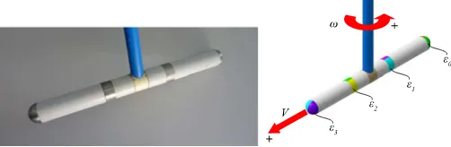
Fig. 1. (Left) Photograph and (right) schematic view of a four-electrode sensor.
addressed but by using the voltage measurements. The voltage mode has been chosen for its simplicity and results were tested on simulations only. On the contrary, in the paper presented here, electronavigation in a group is addressed with current measure-ments, an extension which allows us to test our results both in simulation and experiments. The sensors are slender probes (see Fig. 1), whose technology and models are detailed in [4] and [16], respectively.
This paper aims at exploring the potentialities and the diffi-culties of electric multiagent navigation. In this perspective, we will consider a set of rigid slender probes (or agents) able to move in the same horizontal plane. The motion of each agent is directly controlled using a kinematic model, here reduced to that of a nonholonomic unicycle. Thus, as this is the case in many UVs, the motion of each agent is controlled through the axial velocityV (aligned with the sensor body axis) and the yaw angular velocityω(orthogonal to the plane of the sensors motion).
Based on this framework, we will address the problem of the navigation in formation along with that of the formation shift-ing. In a given formation, the agents have to maintain a spec-ified posture relative to each other. Drawing inspiration from the mormyrid fish, we will impose the following basic rule: two agents cannot emit an electric field at the same time. Based on this rule, we will see how we can elaborate successful control strategies where at each instant each of the passive agents takes a prescribed position in the electric field of the active one, while the role of the active agent of the group rotates over time. It is worth noting here that in order to control the relative position of a passive agent with respect to the active one, we could first seek to invert the model of the passive agent’s electric measure-ments with respect to the position and orientation between the two agents. Unfortunately, this problem poses many difficul-ties, among them, it is nonlinear, sensitive to noise, and does not generally have a unique solution. However, several tech-niques based on optimization or observer control theory have been used with quite good success [17]–[21]. In this paper, we will follow a sensor-based control approach [22], [23]. The ap-proach is based on a direct feedback of the measurements and not, as in the previous approach, on the state variables of a model that represents the world. This kind of approach is well known to the community working in vision. In this context, it is named “visual servo control” [24]. From that point of view, we here propose an “electric servo control,” in which the electric field of the active agent is used as an immaterial prolongation of its body in its surroundings, while the passive agent senses
this electric body in which it seeks to achieve some prescribed measurements preliminarily measured in a specified (desired) relative posture. Unfortunately, the set of poses ensuring the desired measurements cannot be reduced to the desired one, but rather spans a continuous set of poses, named “zero-dynamics” in nonlinear control theory [25]. As a result, this concept will play a crucial role in the subsequent analysis, in particular in all matters concerning closed-loop stability.
This paper is structured as follows. In Section II, we briefly present the model of the electric sensors as well as the available measurements. Section III deals with the locomotion model and in particular, with the effects of nonholonomy of agents (un-deractuated systems). In Section IV, the principles of group navigation in formation are explained. In particular, the con-vergence conditions of the measurements toward their desired values are listed. The zero dynamics, i.e., the internal dynamics with measurement variables forced to their desired values, are given as well as the convergence conditions toward the desired relative posture of the passive agent with respect to the active one. In Section V, one example illustrates in simulation the main properties of the control approach. The problem of switching between formations is addressed in Section VI. In Section VII, our testbed is described and first experiments with two kinds of formation are presented to prove the feasibility of the approach, while switching between formation is also illustrated. Finally, this paper ends with a few concluding remarks and perspectives in Section VIII.
II. MEASUREMENTMODEL
being shifted from agent to agent in a fixed ordered sequence repeated in a continuous loop.
Due to the short range of the sensor [between once (active mode) and twice (passive mode) of the sensor length], the mod-eling problem can be reduced to that of a single pair of neigh-boring agents one being active and the other being passive. To introduce the model of measurements in such a scenario, let us consider the succession of causes and effects, which relate the imposed voltages on the active agent to the measured currents on the passive one.2First, the active agent is set under voltage
through a vector of potentialsU = (U1, U2, . . . Un), imposed on the rings by the voltage generator. OnceU is imposed, the sensor recovers its electric equilibrium by generating an(n×1) vector of currentsI(0)flowing across the rings.3These currents
are given by the intrinsic model of the sensor
I(0)=C(0)U (1)
where C(0) is the (n×n) conductivity matrix of the sensor
when there is no object around it. Second, once the currents are generated on the active agent, they produce in the nearby sensor a basal field, which can be written [16] as
φ(0)(x) = 1
4πγ
Ii(0) ri
(2)
where γ is the conductivity of the (homogeneous) fluid, and ri denotes the distance between the center of theith ring and the pointxat which the potential is evaluated. Third, this basal
field polarizes its nearby surroundings and in particular any pas-sive sensor close to the active one. This polarization generates the vector of 2(n−1) perturbative currents measured by the passive electrodes,4that we simply noteI= (I1, I2, . . . I2n−2)
and which is naturally a function of the pose between the two agents. Due to the slender geometry of the sensor, the measured currents can be written under the following form:
I=Iax +Ilat (3)
where Iax andIlat are called axial and lateral components of the currents. Physically, they correspond to the electric response of the passive agent to its lateral (from left to right) and axial (from rear to front) polarization by the active agent field (2). As shown in Fig. 2, this polarization takes into account the non-negligible interactions of the passive agent body with the active agent field.5 This contrasts with [14], where the voltages were measured while the passive agent body was neglected. The first componentIax is modeled by distributing equally the(n−1) last components of (1) on the 2n−2 half rings after having replaced the components ofUby the values of−φ(0)[given by
2For the sake of clarity, we do not detail the model of electric interactions,
which is the subject of other works progressing in parallel, and refer the reader to the preliminary results [26] where an analytical approach based on the method of refections is applied to the case of complex scenes (several agents, objects).
3The upper index(0)indicates that the quantity is considered without any
object around the sensor [16].
4That is the currents flowing across the2(n−1)half rings.
5Going further into the details, this polarization represents the instantaneous
reconfiguration of the electric charges in order to ensure the electric balance of the passive agent
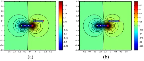
(a) (b)
Fig. 2. Active dipole generates an electric potential, which perturbs the elec-tric currents measured by the electrodes of the passive agent. The differences between the two figures illustrate the influence of the passive agent on the elec-tric field emitted by the active agent. (a) Elecelec-tric potentialφ(0 ). (b) Electric potentialφ.
(2)] evaluated at the center of the rings. The second component represents the lateral response of each ring to the application of the electric field−∇φ(0). It can be modeled by defining a
dipolar tensor of lateral polarization for each ring [16]. Finally, due to the symmetry of the electrodes distribution, the two com-ponentsIax andIlatcan be simply deduced from the vector of measured currentsI by taking for each ring (except the tail), the half-sum and the half-difference of the left and right cur-rents flowing across the symmetric electrodes that constitute this ring. In the following, we will use the(nm ×1)vector of mea-surementsm= (Iax,1, . . . , Iax,n−1, Ilat,1, . . . , Ilat,n−1)T with
nm = 2(n−1),andIax,i, Ilat,iare the axial and lateral currents of theith ring. For example,Iax,1 = I1+2I2 andIlat,1 =I1−2I2.
These measurements obviously depend on the relative posture between the passive and active agents.
III. LOCOMOTIONMODEL OF AGROUP
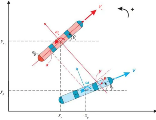
Throughout this paper, the robots are assumed to move in the same horizontal plane. Furthermore, the robots’ motions are modeled using the nonholonomic kinematic model of the uni-cycle. The control inputs are the linear axial velocity V and the angular vertical velocityω(see Fig. 3). When they are con-trolled in formation, the control objective consists of keeping a constant position and orientation (or “relative posture”) between the robots. Following a usual control strategy in multirobot nav-igation [27], one of the robots is distinguished as a “leader,” defining a reference motion for the group. This reference motion is unknown to the other robots or “followers,” and is compatible with the nonholonomic constraints of the kinematic model of locomotion.
Fig. 3. Passive agent (blue) and the active agent (red) are nonholonomic systems. The red electrode is the emitter and blue ones are the receptors. The control objective for the follower agent is to maintain constant values x, y,θ.
passive neighbor. The case of any agent is easily deduced by propagating this basic scenario according to the previous rules. Considering this isolated pair of agents, the relative posture of the passive agent with respect to the active one (here the leader) can be defined in terms of the measurements of the passive agent.
In an absolute frame, the leader posture is(xr, yr, θr), while its velocity is defined by (Vr, ωr). Similarly, the posture of the passive agent in the absolute frame is(xp, yp, θp), and its corresponding velocity(V, ω)defines the two control inputs of the problem:u= (V, ω)T (see Fig. 3). Since these two agents are nonholonomic unicycle systems, we have
⎧
The relative posture of the passive agent in the active agent’s frame is defined by the state vectorX = [x, y, θ]T. With this notation, the objective of the control strategy, defined in the frame of the active agent is to maintainX at a desired value Xd = [xd, yd, θd]T. Our control model is defined by X˙ ex-pressed as a function of the control inputs V and ω of the passive agent. In order to obtain it, let us first write the relation between the relative and absolute postures as
x= (xp−xr) cos(θr) + (yp−yr) sin(θr)
y=−(xp−xr) sin(θr) + (yp−yr) cos(θr)
θ=θp−θr. (5)
Time-differentiating these equations and combining them with (4), we obtain
which takes the form of the following control system: ˙
is a perturbation due to the unknown motion of the active agent. From these considerations, it appears that the formation motion can be perfectly tracked (with X =Xd and X˙ = 0) by the passive agent if, for anyVr,ωr, there exist values ofV andω that satisfy the following constraints:
V cos(θ)−Vr+yωr = 0
Vsin(θ)−xωr = 0
ω−ωr = 0 (8)
the third equation allowing us to defineωdirectly. The desired formationXd = (xd, yd, θd)T is feasible if there exists a value of V that satisfies the two first equations for any Vr, ωr. In particular, a motion along a straight line (ωr = 0, Vr= 0) can be tracked only if θ= 0. To achieve a satisfactory behavior when the leader moves along a straight line, we limit our study to the case whereθd = 0, i.e., to the case where the agents are parallel. Under these conditions, (8) can be satisfied for any motion of the leader agent (i.e., with anyVrandωr) only when θd = 0 and xd = 0. If x=xd = 0, then any turning motion of the leader (ωr = 0) will induce an unavoidable error on the relative posture of the passive agent with respect to the active leader. This point will be further discussed since the formation that we will consider will not satisfyxd = 0.
Since the motion of the passive agent is controlled by two inputs V and ω while three parameters define its evolution, its relative evolution with respect to the active agent can be expressed by the following equation, which is independent of the control
˙
xsin(θ)−y˙cos(θ) =−Vrsin(θ) +yωrsin(θ)−xωrcos(θ). (9) This equation is obtained by combining the two first equations of (6). It represents the nonholonomic constraint imposed to the leader tracking. The control law will not affect this equa-tion, which is independent of the two control inputs V andω. However, it will impose viaV andω, two relations on the three variablesx,y, andθand their derivatives. The control law must be such that these relations, once combined with (9), ensure a stable behavior of the passive agent.
IV. SENSOR-BASEDCONTROLSCHEMES FORMOTION INFORMATION
measure-ments, with no calculation of the relative posture of the leader and follower agents, these methods cannot be directly applied. Nonetheless, they reveal the importance of the choice of the outputs for this kind of system. In our case, the two controlled outputs being two functions of the electric measurements, and since the relative posture of the agents is defined by the three variablesx,y, andθ: an infinite set of relative postures ensuring the desired outputs exists. As a result, the closed-loop dynamics of the system when the outputs are forced to follow their de-sired evolution, i.e., the so called “zero dynamics” of [25], must be studied. Generically, these dynamics are determined by the choice of the outputs, byXd, and by the motion of the leader. In particular, the control outputs must be chosen in order to produce, at least locally, a stable zero dynamics. In our case, de-pending on the curvature of the motion of the active agent, some errors on the relative posture of the controlled passive agent can occur. These points will be detailed in the Section IV-C. Before entering into these details, let us remark that the control schema derived hereafter address the general measurement-based ser-voing problem of an unicycle plant model, and as such, could be extended to other sensors.
A. Principle
As in the case of vision-based control schemes of [24], the control aims at minimizing an error vector e(t) defined as a function of the measurements. Such a vector is here restricted to a linear combination of the measurements:s=Cm(X(t)), whereCis a constant(2×nm)matrix, and
e(t) =Cm(X(t))−sd (10)
where the vectorm(X(t))denotes the vector of measurements (e.g., the electric currents). OnceCis selected, the definition of the control law is straightforward. Indeed, invoking the relation between the state and the control inputs (7) allows one to express the relation between the error and the control inputs as
˙
e(t) =C∂m
∂X(Ju+P(t))−s˙ d(t).
(11)
Then, if we want to assign the following desired behavior to the errore(t):
˙
e(t) =−λe (12)
with a chosen parameterλ>0, we can use the following linear feedback control:
u=−λLe (13)
whereLis a(2×2)matrix of gains.
B. Convergence Condition for the Error e
We now study the convergence of the aforedefined control law. To that end, let us remark that when the vector of desired outputs sd is constant, s˙d = 0, and the active robot is at rest
which ensures that the error decreases if the matrix(C∂ m∂ XJL) is positive definite, i.e., if it satisfies the condition [23]
C∂m ∂XJ
L >0. (15)
To ensure positive definiteness, we propose to take
C∂ m∂ XJ
L= 1 with 1 the identity matrix. This choice leads to the relation
whereLis an estimation of the inverse ofC∂ m
∂ XJ. If the robot stateXwould be known, the classical solution would consist of using the model of measurements to calculate the current value of(C∂ m
∂ X(X)J(X))
−1. However, since the state is unknown (no
observer will be used), this approach is not feasible. Nonethe-less, since a constant relative posture of the passive agent with respect to the active one is desired (X =Xd), one can choose Las(C∂ m∂ X(Xd)J(Xd))−1, whose the value can be calculated
by using the model, or directly measured in a preliminary ex-perimental phase6
or L are singular, then the convergence condi-tions fail and the desired behavior can no longer be guaran-teed. As a result, the choice of C is critical to ensure that
C∂ m∂ X(Xd)J(Xd)
is not singular. Finally, let us remark that since we have for any(2×2)invertible matrixC0, the
invari-ance property
the control law is unchanged by replacingC byC0C, and we
can for instance choose a normalized matrixC.
C. Convergence Condition for the Relative Position Between the Agents
The control law is designed to ensure the convergence of the outpute(t)to zero. Because the dimension of the stateX is 3, while the relative degree of the two independent controlled outputs is 1, the dimension of the zero dynamics is 1. In general, zero dynamics characterize the closed-loop behavior of a con-trolled system [25]. Geometrically, they define a submanifold Zof the state space, which contains all the states of the system such that the controlled outputs are zero, and in particular, the stateXd. Thus, while the convergence of the control law entails that the state tends to reachZ, that does not mean thatX con-verges toXd since the system is underactuated, andZ is not reduced toXd. Therefore, zero dynamicsZmust be studied in
6By imposing small displacements as inputs and measuring the corresponding
Fig. 4. Different configurations of the passive agent belonging toZ, i.e., corresponding to desired output vectorC m(X). The set of the sensor center positionsx, yis represented by the red line. Several corresponding configura-tions of the passive agent are drawn in blue, the desired configuration of the follower agent is in black, and the active agent is in red with a contrasted emitter.
Fig. 5. Relative position of the passive agent x and y belonging to Z (C m(X) =sd) as a function ofθ(top and middle), and the corresponding value ofωr
Vr (bottom). When the active agent moves in a straight line ωr Vr = 0,
the equilibrium position is the desired onex=−0.22m,y=−0.10m, and
θ= 0. When the active agent turns with ωr
Vr =2.61 rd/m, the equilibrium
position is defined byx=−0.2532m,y=−0.041m, andθ=−0.539rd so generating a vector of error:x−xd=−0.0332m,y−yd=0.059 m,
θ−θd=−0.539rd.
detail in order to find out whether the convergence of the outputs to zero does imply the convergence of the state towardsXd, at least locally.
The zero dynamics being spanned by all the possible evolu-tions of the robot when the controlled outputs are identically zero, it is in our case given byZ=
X|Cm(X) =sd
, i.e., a manifold whose analytical construction would require the inver-sion of the model of electric measurements. To circumvent this difficulty, and since the dimension ofZ is 1, the stateX ∈Z can be parametrized byθas:X = [xZ(θ), yZ(θ), θ]T. In doing so, the functions xZ andyZ can be constructed numerically around the desired stateXd 7 as illustrated in Figs. 4 and 5.
Time differentiating this context, the robot velocityX˙ satisfies
7More generallyZcan be parametrized by a single variable. We assume here
thatθis a convenient choice. A parametrization byxoryor any function of the state can be used in a similar way. Parametrization byθimplies thatθis monotonic in the studied subspace ofZaroundθd
in a closed loop (the state of the robot remains inZ) the relation
C∂m(X)
∂X X˙ =CmX˙ = 0 (19)
whereCm =C∂ m∂ X(X) will denote a(2×3)matrix ofrank= 2. Assuming that the left(2×2)submatrixCm1ofCmis invert-ible, and denoting the right(2×1)submatrix ofCm byCm2,
the velocities will verify in a closed loop the simple relation
˙ x ˙ y
=−Cm−11Cm2θ˙ (20)
which can be rewritten as8
˙
x=Zx(θ) ˙θ
˙
y=Zy(θ) ˙θ. (21)
The control law allowing the maintenance of the state of the robot in Z, its velocity X˙ will necessarily satisfy (21). Since the two agents are nonholonomic, depending on the motion of the leader, it is possible that the state of the follower does not tend toward the desired state. In fact, as already discussed in Section III, the behavior of the follower robot is governed by (9), which once combined with (21), gives
Zx(θ) ˙θsin(θ)−Zy(θ) ˙θcos(θ)
=−Vrsin(θ) +yZ(θ)ωrsin(θ) +xZ(θ)ωrcos(θ). (22)
This equation describes the closed-loop behavior of the follower agent as a function ofθandθ˙only. It plays a crucial role in all the following. In particular, it will reveal the motions of the follower robot in a closed loop. Using this result, we are now able to address the question of whether the agent will be steered to the desired stateXd (or equivalentlyθd) or not, and if this is the case, will it remain in that desired state? In order to address this question, we will consider (22) in two cases. First, when the leader is moving in a straight line (see Section IV-C1) and second, when the leader is turning (see Section IV-C2).
1) Leader Moves in a Straight Line (ωr= 0): Equation (22) then becomes
Zx(θ) ˙θsin(θ)−Zy(θ) ˙θcos(θ) =−Vrsin(θ) (23)
whose obvious solution is given by ( ˙θ=θ= 0). Thus, θ= θd = 0(and so anyX =Xd) is an equilibrium state. Further-more, the first-order linearization of (23) around the desired stateθd
˙ θ− Vr
Zy(θd)
θ= 0 (24)
defines the local behavior of the follower agent. A simple anal-ysis of (24) leads to the following four conditional conclusions.
a) If Vr
Zy(θd) <0, thenθwill converge toward zero. Therefore,
xandywill converge towardxd andyd ifX =Xd is the unique state belonging toZwithθ= 0.
8By definitionZ
x = ∂ x
Z
∂ θ andZy = ∂ yZ
∂ θ , but the analytical expression of
b) If Vr
Zy(θd) >0, thenθwill diverge and consequentlyxand
ywill diverge too. c) If Vr
Zy(θd) = 0, then neitherθchanges nor doxory. The
passive agent does not move. The error if it exists, remains unchanged.
d) SinceVr appears in ZyV(rθd), if the chosen formation and
outputs are such that the control law is stable forVr >0, then the same control law will be unstable forVr <0. Consequently, in order to ensure that a formation can go backward, a new set of controlled outputs has to be defined. 2) Leader Turns (ωr = 0): In this case, we will consider two subcases depending on whetherxd is equal to zero or not:
a) Ifxd = 0, all the desired motions are feasible (indepen-dently ofωrandVr). Thus, anyX =Xd(withθ=θd = 0 andx=xd = 0) is an equilibrium state for (22). More-over, the local behavior of the passive agent is governed by the first-order expansion of (22) around the desired state Xd
Thus, similar conditions to those met in the previous case can be stated, except that the critical velocity is no longer Vr but rather
Consequently, to ensure stability, the critical value of the forward velocity now depends onωr,yd andZx(Xd). b) Ifxd = 0, the equilibrium state for (22) is no longerθd
but a different state denotedθe, and such that
−Vrsin(θe) +yZ(θe)ωrsin(θe) +xZ(θe)ωrcos(θe) = 0 (27) whenθeexists. If for a given value of the turning curvature
ωr
Vr, (27) has no solutionθ
e, then the motion of the passive
agent cannot be stabilized and there is no equilibrium. On the other hand, when (27) has a solutionθe, the first-order expansion of (22) around this equilibrium state can be written as
Finally, three conditional conclusions arise.
1) IfVr >0andβα >0, thenθwill converge towardθeandx andywill converge towardxeandye.(θe, xe, ye)defines the posture of the passive agent with respect to the active one whenωr = 0.
2) Forωr
Vr = 0, (28) is reduced to (24). Sinceθ
e= 0, we have
α=−Zy(θe)andβ= 1.
3) The condition of stability is based on |ωr
Vr| and on the
property of the equilibrium point defined by the choice of the output (which affectsZ).
Note that we have hitherto assumed that P(t) = 0in (11). However, in reality, the motion of the active agent will produce
a perturbationP(t)= 0that will generate an unavoidable mea-surement error. Moreover, in a transient maneuver where the robots move in order to configure the group in a given forma-tion (see Secforma-tion VI),s˙d = 0, and the measurement error is then governed by
As a result, a small error in position will be induced too. Finally, the proposed control strategy will be tested in simulation in Section V and in experiments in Section VII.
V. EXAMPLE OFMOTION INFORMATION
For the purpose of illustration, a formation of four identical agents is considered. The relative posture between two neigh-bors isXd = (xd, yd, θd) = (−0.22,−0.10,0) (in meters and radians).
A. Choice of Control Outputs
In this desired configurationXd, considering only one active agent and its passive neighbor, the vector of measurements of the passive agent ism= [Iax,1,Iax,2,Iax,3,Ilat,1,Ilat,2,Ilat,3]T
= 1.10−4[0.315,−0.357,−0.645,0.106,0.317,0.499], while
its Jacobian matrix is
Examining this matrix, it appears that many combinations of the outputs can be chosen to obtain a nonsingular matrixC∂ m∂ XJ. In the following, we choose as control outputsIax,3andIax,1−
Iax,2 (i.e.,C∂ m∂ XJ = 1.10−3
to the conditional conclusions of Section IV-C, we have two cases depending on wether the leader moves in a straight line withVr >0, or turns along a path of curvatureωr/Vr. In the first case, the stability is ensured ifZy(θd)<0[see (22), with Zydefined by (21)], a condition which is verified by our chosen outputs, since in this caseZy(θd) =−0.1370<0. In the second case, sincexd = 0, there exist some errors on the relative posture of the follower (see Section IV-C2).
Then, the control will force the follower agent to reach the zero dynamics manifoldZ(=
X|Cm(X) =sd
). As a result, the knowledge ofZ is essential. In particular, imposing a ro-tation of the leaderωr= 0 will change the robot position on Z. Fig. 4 illustrates the states of the follower agent belonging toZ. Another representation of the zero dynamics manifold is given in Fig. 5. In this case, the two upper plots numerically define the functionsxZ(θ)andyZ(θ). The lower plot defines the equilibrium state onZ for different curvature of the leader motion. It shows ωr
Fig. 6. Two eigenvalues ofC∂ m ∂ XJ
Linvolved in the convergence condition (15) (top), and βα involved in (28) as a function of ωr
Vr for configurations
belonging toZ(bottom).
allow us to fully determine the relative position of the two agents when the control law is stable.9As regards the stability of the closed-loop dynamics, it is conditioned by the sufficient condi-tion (15) along with the stabilizacondi-tion of (28) onθe. In the upper part of Fig. 6, the two eigenvalues of
C∂ m∂ XJ
Lare plotted for the equilibrium configuration corresponding to the curvature of the leader path defined by ωr
Vr. On the upper part of Fig. 6, the
term βα involved in (28) is plotted under the same conditions.βα has to be positive to ensure that the passive agent does follow the active one withVr >0. Based on these plots, a stable be-havior is obtained when the leader agent follows a path with a curvature such that−5rd/m< ωr
Vr <5.35rd/m.
B. Simulation
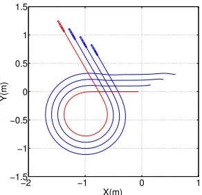
The leader agent is subject to a motion composed of different phases. The leader is initially motionless (phase A, fromt= 0to 5 s), then it follows a straight line with a linear velocityV =0.05 m/s (phase B, fromt= 5to 20 s). During the phase C (from t= 20to 30 s), the angular velocity smoothly increases up to reach a constant value of 0.13 rd/s during phase D (fromt= 30 to 60 s), where the leader follows a circle of curvature ωr
Vr =
2.61 rd/m. A symmetric evolution of the velocity of the leader is then imposed. In this case, the angular velocity decreases during phase E (t= 60to 70 s), then a straight line is followed during phase F (t= 70to 95 s) and the leader stops in the final phase G (t= 95to 100 s). As illustrated in Fig. 7, the formation is stably maintained throughout the entire motion. However, as the curvature increases, errors with respect to the relative positions increase.
The initial posture of the passive agent being biased by errors (see Fig. 8), the initial measurements do not coincide with the desired onese(0)= 0, and the control law quickly nullifies the measurement error during the phase A so ensuring the passive agent to reach the zero dynamics Z. However, since Vr= 0, an error on the position remains. In phases B and F, while the
9Indeed, for any value ofω
r/Vr, the lowest plot of Fig. 5 gives the corre-sponding value ofθ, while the two others givex(θ)andy(θ)and finally define the point onZtoward which the state converges.
Fig. 7. Paths followed by four agents illustrate the stability of the formation, even if the leader (red) has a complex motion with various curvatures.
Fig. 8. Results for the first follower agent are presented in the first column, while for the last one the results are in the second column. All the curves are presented as a function of time. In the first line, the error on the controlled measurements is shown. In the second line the error on the relative position are presented and in the last line the control inputV ω(solid line) and the velocity of the active agentVrωr (dotted line) are drawn.
leader moves along a straight line withVr >0, one observes the convergence of the robot posture toward the desired value x−xd = 0,y−yd = 0,andθ= 0.
Due to the nonzero distance between agents along thex-axis, a nonzero error on the relative position of the passive agent necessarily occurs for a leader following a curved motion [see equation (8)]. This is confirmed in Fig. 8 during phases C, D, and E, where nonnegligible posture errors can be observed, while the measurement errors are very small. During phase D, the velocity of the leader is defined by Vr =0.05 m/s, and ωr=0.13 rd/s; thus, its curvature is ωVrr =2.61 rd/m, and its follower converges toward the equilibrium posture defined in Fig. 5. In Fig. 5, the red dotted line defines the equilibrium point corresponding to this curvature of the leader path. As indicated on these plots, when the second agent is the follower, the equilibrium point corresponding to ωr
Vr =2.61 rd/m isx=
ωr =0.131 rd/s). Therefore, its curvature isωVrr =1.66 rd/m and the position error of the last agent with respect to its neighbor is reduced (see Fig. 5).
Due to the leader motion (P(t)= 0), small errors on they position and on the measurements persist when the leader is not stopped.
VI. SENSOR-BASEDCONTROLSCHEMES FOR FORMATIONSWITCHING
Since different formations can be used, it is useful to be able to switch between them. This is achieved by changing the relative desired position of the passive agent with respect to the active one.
A. Statement of the Problem
To tackle the difficulty of the agents, nonholonomy, a refer-ence motion (or “maneuver”) is first defined in order to steer a virtual agent from the initial desired postureXd1 to the final
oneXd2. To that end, the active agent is kept fixed, while in
its frame, the motion of the virtual passive agent is defined by Xv = [xv(t), yv(t), θv(t)]T, with agent measure the currents produced by the active agent, which are gathered intomv(Xv(t)).
B. Control Law
Based on direct electric measurements, the control law aims at making the real passive agent track the maneuver of the virtual passive agent. To that end, the choice has been made to control the measurement error
e(t) =Cm(X(t))−Cmv(Xv(t)). (32)
Differentiating the above relation with respect to time and com-bining it with the model (7) (withVr =ωr = 0since the active Since the expected value forXisX =Xv(t), the estimation of
C∂ m∂ X(X)J(X)can be replaced byC∂ m(∂ XXv(t))J(Xv(t)) which is known. As a result, the control law becomes
u=−λLve(t) +uv(t) (35)
which generalizes (13) from formation maintaining to forma-tion tracking. Thus, as in Secforma-tion IV, a condiforma-tion of conver-gence on the error measurement is given by (15) withLv =
(C∂ m∂ X(Xv)J(Xv)) −1
. This condition implies that (C∂ m∂ XJ)is not singular throughout the entire maneuver. Since the passive agent moves with respect to the active one (Xv(t)is not con-stant), this condition is more difficult to satisfy than in the case of formation maintaining. Finally, even if the proposed control law allows us to deduce the desired value for the measurement, the motion of the robot remains unknown.
C. Condition of Stability
Both the virtual and real agents are nonholonomic systems (9), whose movements satisfy the constraints
Being interested in the difference between the motion of the virtual and the real agent, we define the vectordX=X−Xv. A first-order expansion of (36) arounddX = 0, combined with (31), gives the following constraint on tracking errors (between the virtual and real agents):
dx˙sin(θv)−dy˙cos(θv) +Vvdθ= 0 (37)
which models the nonholonomy of the agents. As expected, the control law is designed to ensure that the controlled measure-ments of the real agent match those of the virtual one. Thus, withCm =C∂ m∂ X(X), we have
Cm(X(t)) =Cm(Xv(t))
Cm(X(t)) ˙X =Cm(Xv(t)) ˙Xv(t). (38)
Since our objective is to satisfy dX= 0 (i.e., the real agent tracks the virtual one), we study the linearized evolution ofdX arounddX = 0. To that end, we linearize (38) arounddX= 0
Starting from (39) and using similar notation and calculation to those used in (20) and (21), allows one to parameterize the evolution of the tracking error as a function of(dθ, dθ)˙ only
⎧
Fig. 9. Electrolocation test bench.
and obtain the evolution equation ofdθ
(Zx(Xv) sin(θv)−Zy(Xv) cos(θv))dθ˙
+ (Vv+vxsin(θv)−vycos(θv))dθ= 0 (41)
from which we deduce the following three cases.
1) Starting fromdθ=dθ˙= 0ensures a perfect tracking of the virtual agent motion by the real agent.
2) IfVv+vx(Xv,X˙v) sin(θv)−vy(Xv,X˙v) cos(θv) = 0, which occurs, for example, when the virtual agent stops, then the error will be kept constant.
3) If γ=Vv+vx(Xv,X˙v) sin(θv)−vy(Xv,X˙v) cos(θv)
Zx(Xv) sin(θv)−Zy(Xv) cos(θv) >0, the
motion of the real agent will converge to the motion of the virtual agent.
For a desired motion of the virtual agent, the controlled measurement Cm(t) will be chosen to avoid singularity of C∂ m
∂ X(X
v(t))J(Xv(t))and to ensureγ >0.
VII. EXPERIMENTS
A. Electrolocation Testbed
In order to test our sensors [4] and algorithms under controlled and repeatable conditions, an automated test bench consisting of a cubic tank of 1 m side with insulating walls, filled with fresh water, and a three-axis cartesian robot has been built (see Fig. 9). The robot fixed on top of the aquarium allows probes positioning in translation along X andY with a precision of 1/10mm and the orientation in the(X, Y) plane is adjusted in0.1◦ using an absolute yaw-rotation stage. The two agents tested are positioned in the aquarium at adjustable height using a rigid perch. This vertical insulating tube allows the passage of electrical cables dedicated to the signals coming from the electrodes to readout electronics (analog chain + ADC board) without compromising the measurements. The maximum speed available is 0.3 m/s (≃1km/h) for both translations and 1.4 rd/s (13.5 r/m) for rotation.
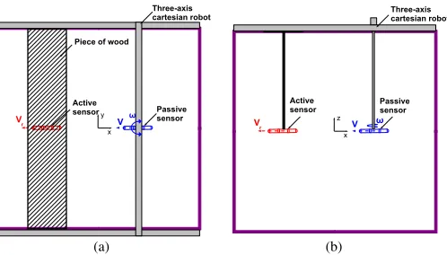
Two slender probes (or agents) of 22 cm each are used. One is active and the other is passive (see Fig. 10). The active agent is attached to a piece of wood via a vertical rod. The piece of wood can be translated along the tank by a hand so producing a straight line motion of the leader, parallel to theX-axis [see Fig. 10(a)]. In all experiments, the basal field of the active agent is generated by a sine wave voltage with a frequency 22.5 KHz and an amplitude of 5 V. As regards the passive probe, it is attached to the Cartesian robot (gantry) and motion-controlled
(a) (b)
Fig. 10. Experimental test bench, the allowed motion of the active sensor is the straight line and the motion of passive sensor is nonholonomic. (a) Test bench top view. (b) Test bench side view.
via the control inputsu= [V, ω]T based on the electric currents feedback. Both agents are in the same horizontal plane. The sampling period of the bench isTe=0.015 s.
To illustrate the control laws in our tank, we now report the results of three experiments. In the first two experiments, the active agent moves in a straight line, while the passive one follows it in order to maintain a given relative configuration withyd = 0in the first case, andyd = 0in the second (in the second case the two agents are aligned). The third experiment consists of switching between the two previous configurations (from a formation where the two probes are aligned to another where they are not), while the active agent is kept fixed. For all experiments, the speed of convergence of the error dynamics
is such thatλ=0.7, while the matricesC, ∂ m(X
d)
∂ X andLare precomputed with simulations on our fast analytic simulator. All the desired measurementsm
Xd
are experimentally measured in a preliminary phase that allows emancipating ourselves from the influence of the conductivity fluctuations.
B. First Motion in Formation
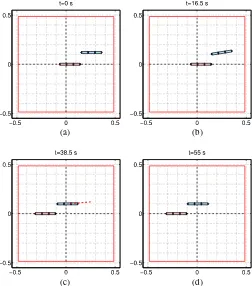
The desired posture of the follower in the leader frame is fixed toxd =−0.22m,yd =−0.10m, andθd = 0as in Section V. We define a motion of the leader in three phases. In Phase A, the leader is at rest and the follower is positioned in the leader frame with an initial error. In Phase B, we move the leader (Vr >0, ωr≃0). In Phase C, the leader is stopped.
In Fig. 11, the evolutions of the leader and follower are shown. Fig. 12 shows the control input, the measurement error and the error on the relative position between agents10
Att= 0, a small error on the initial position of the passive agent (y−yd =−0.02m [see Fig. 11(a)–12(b)]) produces an error on the measurements [see Fig. 12(a)]. Between 0 and 16.6 s (Phase A) the leader is at rest (Vr =ωr= 0) and the control law of the follower produces a velocity u [see Fig. 12(c)] that nullifies the measurement error [see Fig. 12(a)]. The control law forces the relative posture of the passive agent,
10The motion of the passive agent is known in an absolute frame via the
(a) (b)
(c) (d)
Fig. 11. Experimental results. (a)–(d) describe the different phases of motion for the leader (left) and the follower (right) in the tank, red dashed line in (c) indicated the positions of the follower center during the Phase B.
to reach the zero dynamics manifoldZ. The relative posture is stable but since Vr = 0, it is not the desired one. In other terms, an error on the relative position remains [see Fig. 11(b)– 12(b)]. At 12 s, due to handling of the support of the leader, an intentional perturbation is generated and rejected by the control law. As a results, the follower stabilizes its posture in a slightly different state belonging toZ. Between 16.6 and 38.6 s (Phase B), we move manually the leader via its support, in a straight line (Vr>0andωr ≃0). During this phase the position error decreases [see Fig. 11(c)–12(b)] and the posture of the follower converges toward the desired posture. A small measurement error occurs due to the motion of the leaderP(t)= 0. Between 38.6 and 60 s (Phase C), the leader is stopped (Vr =ωr = 0), the control of the follower allows us to nullify the measurement error [see Fig. 11(d)–12(a)] and the passive agent remains in the desired formation.
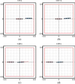
C. Motion in the Single File Formation
The purpose of this experiment is to test the single file for-mation. The desired relative posture of the follower is fixed to xd =−0.32m,yd =θd = 0.
The matrixCis defined according to a methodology where the desired zero dynamics is imposed [32]. Applying this approach, the matrixCis
C=
−0.987 −0.131 −0.037 −0.083 −0.017 0.013 −0.069 0.003 −0.004 0.908 −0.412 0.037
.
(a)
(b)
(c)
Fig. 12. Experimental results for the follower agent. (a) Error on the con-trolled measurements. (b) Error on relative position. (c) Control inputV,ω. The abscissa is the time (s).
(a) (b)
(c) (d)
Fig. 13. Experimental results. (a)–(d) describe the different phases of motion for the leader (left) and the follower (right) in the tank, red dashed line in (c) indicates the positions of the follower center in the Phase B.
position error during Phase B. For this test, we haveZy =6.2, and the relative position error does not reach zero during phase B.
Between 28.1 and 40 s (Phase C), the leader is stopped (Vr=ωr = 0), while the control law nullifies the measurement error [see Fig. 13(d)–14(a)]. However, the relative position error remains constant.
D. Change of Formation
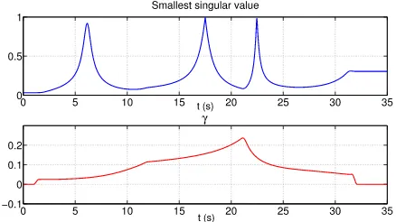
This experiment addresses the problem of switching between the two formations previously studied. This maneuver is defined by the motion of a virtual agent going from the initial posture (xd =−0.32myd =θd = 0), where it is aligned with the ac-tive real agent, to the final posture (xd =−0.22myd =−0.10 mθd = 0), which corresponds to the desired formation studied in Section VII-B. The maneuver is defined by using the simula-tion which allows us to precompute the feedforward component uv of (35). The corresponding trajectory is represented in blue in Fig. 15, its duration is 35 s. This maneuver is obtained with a constant linear velocityVv =0.005 m/s and a variable an-gular velocityωv defined in Fig. 17(c). Based on the current measurements feedback, the control objective consists of mak-ing the passive agent track the motion of the virtual agent. To control the passive agent, two controlled outputs are defined by the matrix C. These outputs have to satisfy the following conditions:
1) C∂ m∂ XJ has no singularity throughout the motion; 2) γ >0.
(a)
(b)
(c)
Fig. 14. Experimental results for the follower agent. (a) Error on the controlled measurements. (b) Error on the relative position between the leader and the follower. (c) Control inputV,ω. The abscissa is the time (s).
We choose the matrixCin such a way that when the virtual agent has the positionAof Fig. 14 (att=17.5 s), we have
C∂m(X v(A))
∂X J(X
v(A)) = 1
(42)
where 1 is the(2×2)identity matrix, while the matrixCis the Moore–Penrose pseudoinverse of∂ m∂ X(Xv)J(Xv).
For the given maneuver
C=
0.0478 −0.137 0.154 −0.076 0.058 0.0098 0.4126 −1.09 1.066 −0.589 0.455 0.092
and the smallest singular value ofC∂ m(∂ XXv(t))J(Xv(t)),and γare drawn in Fig. 16. The conditions of stability are fulfilled along the maneuver.
(a) (b)
Fig. 15. Experimental results. (a) Path followed by the sensor (red line) and the virtual agent (blue line), the virtual agent has a complex motion, the real passive agent follows this motion (maneuver). The active agent is fixed (left). (b) Zoom view of the path followed by the passive (red dashed line) and virtual agent (blue line).
Fig. 16. Verification of the stability requirements of the maneuver. Smallest singular value ofC∂ m(∂ XXv(t))J(Xv(t))
(top) and values ofγ (bottom) along the maneuver.
After this simulation phase, the desired maneuver is exper-imentally played in an open loop in order to record the ex-perimental measurement of the virtual agentmv(Xv). This is achieved with a downsampling of 16 and a linear interpolation which generates the points between two samples. This process allows one to generate a file with the parameters (Lv,uv and mv(Xv)) that will be used in the further experiments.
The initial position of the passive agent presents a small initial error on relative position. The desired motion of the virtual agent starts with a small delay (2.9 s) (Phase A) and stops before the cut-off (Phase C) of the control law. This allows one to observe the motion of the follower (Phase B) beyond the maneuver. The path followed by the sensor (red line) is shown in Fig. 15. Between 0 and 2.9 s (Phase A), the virtual agent is at rest, and the control law of the follower produces an initial velocity u [see Fig. 17(c)], which nullifies the measurement error [see Fig. 17(a)]. Due to the stabilization of the real agent posture in a state belonging toZ, it has a position errorX− Xv = (−0.004m,0,−4◦)[Fig. 17(b)]. Between 2.9 s and 33.8 s
(Phase B), Fig. 17(c) shows that the real agent velocity does track that of the virtual one. This is achieved with small transitory oscillations, which are produced by the feedback component of (36). Between 33.8 s and the end (Phase C), the virtual agent is at rest and the relative position error remains constant [see Fig. 17(b)].
(a)
(b)
(c)
(d)
Fig. 17. Experimental results in the case of switching formation. (a) Error on the controlled measurements. (b) Error on the relative position and orientation between virtual and real agents. (c) Control input(V, ω)(solid) and velocity (Vv, ωv)of the virtual agent (dotted). (d) Relative position of the real agentX (blue) and the virtual agentXv(red) in the active agent frame.
VIII. CONCLUSION
Coordinated underwater navigation of a group of vehicles close to each other is a challenging task for underwater robotics. In this paper, we address this problem by way of bioinspiration and present first theoretical and then experimental results on underwater multirobot navigation using the electric sense. The approach is based on a sensor recently described in [4]. By combining rules inspired by electric fish with a follower-leader multiagent strategy, we have addressed the problem of navi-gating while maintaining a given formation of a group of non-holonomic swimmers. The control strategy is based on the direct servo control of the electric measurements. Sufficient conditions of convergence of the control law, in the case of nonholonomic agents, have been developed. The critical bounds, which condi-tion the possible mocondi-tion of the leader (especially those related to the path curvature) have also been pointed out along with the importance of the choice of the controlled outputs on the sta-bility of the control. Based on a servoing of the measurements, the control strategies are especially adapted to the motion of a group of robots in a given formation since in this case constant electric measurements are desired. The proposed approach has the advantage of avoiding the resolution of the inverse problem of the electric measurements with respect to the relative inter-agent posture. As a consequence, the control laws require very few computations. Some errors in the relative posture between the passive and active agents appear in the case of a leader fol-lowing a curved path. The case of transient maneuvers steering the swarm toward a given formation is also addressed using an extension of the formation maintaining control in the case of the tracking of a virtual agent motion based on the electric mea-surements feedback. These control strategies have been tested experimentally and show results in good accordance with the theoretical analysis. Even if to date, our testbed does not allow us to experiment complex motions of the leader, the feasibility of the approach is validated. The next step will be to experiment with this approach on real autonomous agents in a larger tank, and to mix this approach with the reactive controllers of [33] and [34] devoted to obstacle avoidance, in order to produce stable navigation strategies adapted to complex environments.
REFERENCES
[1] A. Kalmijn, “Electro-perception in sharks and rays,”Nature, vol. 212, no. 5067, pp. 1232–1233, 1966.
[2] M. MacIver and J. Solberg, “Towards a biorobotic electrosensory system,”
Auton. robots, vol. 11, pp. 263–266, 2001.
[3] M. MacIver, E. Fontaine, and J. Burdick, “Designing future underwater vehicles: Principles and mechanisms of the weakly electric fish,”IEEE J. Ocean. Eng., vol. 29, no. 3, pp. 651–659, Jul. 2004.
[4] N. Servagent, B. Jawad, S. Bouvier, F. Boyer, A. Girin, F. Gomez, V. Lebastard, C. Stefanini, and P.-B. Gossiaux, “Electrolocation sensors in conducting water bio-inspired by electric fish,”IEEE Sens. J., vol. 13, no. 5, pp. 1865–1882, May 2013.
[5] (2013). Demonstrations of the Angels platform, [Online]. Available: http://www.youtube.com/watch?v=HoJu0OLyW4o
[6] C. D. Hopkins, “Electrical perception and communication,” in Encyclo-pedia of Neuroscience. New York, NY, USA: Oxford, 2009, vol. 3, pp. 813–831.
[7] S. A. Stamper, E. Carrera-G, E. W. Tan, V. Fug`ere, R. Krahe, and E. S. Fortune. (2010). “Species differences in group size and
sory interference in weakly electric fishes: Implications for electrosen-sory processing,” Behav. Brain Res. [Online]. 207(2), pp. 368–376. [Online]. Available: http://www.sciencedirect.com/science/article/pii/ S0166432809006317
[8] T. Bullock, R. Hamstra, and H. Scheich, “The jamming avoidance response of highfrequency electric fish, Part I and II,”J. Comp. Physiol., vol. 77, pp. 1–48, 1972.
[9] W. Heiligenberg,Neural Nets in Electric Fish. Cambridge, MA, USA: MIT Press, 1991.
[10] S. Stamper, M. Madhav, N. Cowan, and E. Fortune, “Beyond the jamming avoidance response: weakly electric fish respond to the envelope of social electrosensory signals,”J. Exp. Biol., vol. 215, no. 23, pp. 4196–4207, 2012.
[11] S. Schumacher and G. von der Emde, “Jamming avoidance during ac-tive electrolocation of objects in the weakly electric fish, gnathonemus petersii,” inFront. Behav. Neurosci. Conf. Abstract: Tenth Int. Congr. Neuroethol., 2012, doi: 10.3389/conf.fnbeh.2012.27.00230.
[12] K. Gebhardt, M. B¨ohme, and G. von der Emde, “Electrocommununica-tion in social groups of weakly electric fish: A comparison of mormyrus rume and marcusenius altisambesi (mormyridae, teleostei),” inFront. Be-hav. Neurosci. Conf. Abstract: Tenth Int. Congr. Neuroethol., 2012. doi: 10.3389/conf.fnbeh.2012.27.00235.
[13] A. Caputi, R. Budelli, and C. Bell, “The electric image in weakly electric fish: Physical images of resistive objects in gnathonemus petersii,”J. Exp. Biol., vol. 201, no. 14, pp. 2115–2128, 1998.
[14] C. Chevallereau, F. Boyer, V. Lebastard, and M. Benachenou, “Electric sensor based control for underwater multi-agents navigation in formation,” inProc. IEEE Int. Conf. Robot. Autom., 2012, pp. 1161–1167.
[15] Y. Morel, M. Porez, and A. Ijspeert, “Estimation of the relative position and coordination of mobile underwater robotic platforms through electric sensing,” inProc. IEEE Conf. Robot. Autom., 2012, pp. 1131–1136. [16] F. Boyer, P. Gossiaux, B. Jawad, V. Lebastard, and M. Porez., “Model
for a sensor bio-inspired from electric fish,”IEEE Trans. Robot., vol. 28, no. 2, pp. 492–505, Apr. 2012.
[17] J. Solberg, K. Lynch, and M. MacIver, “Active electrolocation for under-water target localization,”Int. J. Robot. Res., vol. 27, no. 5, pp. 529–548, 2008.
[18] J. Solberg, K. Lynch, and M. MacIver, “Robotic electrolocation: Active underwater target localization,” inProc. Int. Conf. Robot. Autom., 2007, pp. 4879–4886.
[19] G. Baffet, F. Boyer, and P. Gossiaux, “Biomimetic localization using the electrolocation sense of the electric fish,” inProc. IEEE Robot. Biomimet., 2008, pp. 659–664.
[20] V. Lebastard, C. Chevallereau, A. Amrouche, B. Jawad, A. Girin, F. Boyer, and P. Gossiaux, “Underwater robot navigation around a sphere using electrolocation sense and kalman filter,” inProc. IEEE Int. Conf. Intell. Robots Syst., 2010, pp. 4225–4230.
[21] V. Lebastard, C. Chevallereau, A. Girin, N. Servagent, P.-B. Gossiaux, and F. Boyer, “Environment reconstruction and navigation with electric sense based on a Kalman filter,”Int. J. Robot. Res., vol. 32, pp. 172–188, 2013. [22] C. Samson, M. Le Borgne, and B. Espiau,Robot Control: the Task
Func-tion Approach. Oxford, U.K.: Oxford Science, 1991.
[23] B. Espiau, F. Chaumette, and P. Rives, “A new approach to visual servoing in robotics,”IEEE Trans. Robot. Autom., vol. 8, no. 3, pp. 313–326, Jun. 1992.
[24] F. Chaumette and S. Hutchinson, “Visual servo control—Part I: Basic approaches,”IEEE Robot. Autom. Mag., vol. 4, no. 13, pp. 82–90, Dec. 2006.
[25] A. Isidori,Nonlinear Control Systems. 3rd ed. Berlin, Germany: Springer-Verlag, 1995.
[26] P.-B. Gossiaux, M. Benachenhou, V. Lebastard, B. Jawad, M. Porez, and F. Boyer, “Multi-agents electric simulator,” Report D2.5, The ANGELS project, European Commission Future and Emerging Technologies (FET) contract number: 231845, 2011.
[27] N. E. Leonard and E. Fiorelli, “Virtual leaders, artificial potentials and coordinated control of groups,” inProc. 40th IEEE Conf. Decis. Contr., Orlando, FL, USA, Dec. 2001, pp. 2968–2973.
[28] C. Samson, “Time-varying feedback stabilisation of car like wheeled mo-bile manipulator,”Int. J. Robot. Res., vol. 12, no. 1, pp. 55–64, 1993. [29] J. Desai, J. Ostrowski, and V. Kumar, “Controlling formations of multiple
mobile robots,” inProc IEEE Int. Conf. Robot. Autom., 1998, vol. 4, pp. 2864–2869.
[30] T.-C. Lee, K.-T. Song, C.-H. Lee, and C.-C. Teng, “Tracking control of unicycle-modeled mobile robots using a saturation feedback controller,”
[31] M. Egerstedt and X. Hu, “Formation constrained multi-agent control,”
IEEE Trans. Robot. Autom., vol. 17, no. 6, pp. 947–951, Dec. 2001. [32] M. Benhachenhou, C. Chevallereau, V. Lebastard, and F. Boyer,
“Syn-thesis of an electric sensor based control for underwater multi-agents navigation in a file,” inProc. IEEE Conf. Robot. Autom., 2013, pp. 4608– 4613.
[33] V. Lebastard, F. Boyer, C. Chevallereau, and N. Servagent, “Underwater electro-navigation in the dark,” inProc. IEEE Conf. Robot. Autom., 2012, pp. 1155–1160.
[34] F. Boyer, V. Lebastard, C. Chevallereau, and N. Servagent, “Underwater reflex navigation in confined environment based on electric sense,”IEEE Trans. Robot., vol. 29, no. 4, pp. 945–956, Aug. 2013.
Christine Chevallereau(M’13) received the Grad-uation degree and the Ph.D. degree in control and robotics from Ecole Nationale Sup´erieure de M´ecanique, Nantes, France in 1985 and 1988, respectively.
Since 1989, she has been with the CNRS, Institut de Recherche en Communications et Cybernetique de Nantes. Her research interests include modeling and control of robots of manipulators and locomo-tors robots and bioinspired robotics.
Mohammed-R´edha Benachenhou was born in Alg´erien, Algeria, in 1988. He received the Master’ degree in automatics from the University of Science and Technology of Oran, Algeria, in 2010. He is cur-rently working toward the Ph.D degree with Ecole Centrale de Nantes, Nantes, France, where he works with the Robotics Team, Institut de Recherche en Communication et Cybern´etique de Nantes.
Vincent Lebastard(M’12) was born in France in 1977. He joined the ´Ecole Normale Sup´erieure de Cachan, France, in 2001 and received an aggregation from the Ministry of the Education in Electrical En-gineering in 2002. He received the Ph.D degree from the University of Nantes, Nantes, France, in 2007.
He is an Assistant Professor with ´Ecole des Mines de Nantes and a member of Institut de Recherche en Communication et Cybern´etique de Nantes. His research interests include biorobotics and nonlinear control and observation.
Fr´ed´eric Boyerwas born in France in 1967. He re-ceived the Diploma degree in mechanical engineering from the Institut National Polytechnique de Greno-ble, GrenoGreno-ble, France, in 1991; the Masters degree in mechanics from the University of Grenoble in 1991; and the Ph.D. degree in robotics from the University of Paris VI, Paris, France, in 1994.
He is currently a Professor with the Department of Automatic Control, Ecole des Mines de Nantes, Nantes, France, where he works with the Robotics Team, Institut de Recherche en Communication et Cybern´etique de Nantes (IRCCyN). His current research interests include struc-tural dynamics, geometric mechanics, and biorobotics.