R and Data Mining: Examples and Case Studies

(1)

R and Data Mining: Examples and Case Studies

1 Yanchang Zhao

yanchang@rdatamining.com

http://www.RDataMining.com

April 26, 2013

1

(2)

Case studies: The case studies are not included in this oneline version. They are reserved ex-clusively for a book version.

Latest version: The latest online version is available athttp://www.rdatamining.com. See the

website also for anR Reference Card for Data Mining.

R code, data and FAQs: R code, data and FAQs are provided athttp://www.rdatamining. com/books/rdm.

Chapters/sections to add: topic modelling and stream graph; spatial data analysis. Please let me know if some topics are interesting to you but not covered yet by this document/book.

Questions and feedback: If you have any questions or comments, or come across any problems

with this document or its book version, please feel free to post them to the RDataMining group

below or email them to me. Thanks.

Discussion forum: Please join our discussions on R and data mining atthe RDataMining group <http://group.rdatamining.com>.

Twitter: Follow @RDataMining on Twitter.

(3)

List of Figures

3.1 Histogram . . . 12

3.2 Density . . . 13

3.3 Pie Chart . . . 14

3.4 Bar Chart . . . 15

3.5 Boxplot . . . 16

3.6 Scatter Plot . . . 17

3.7 Scatter Plot with Jitter . . . 18

3.8 A Matrix of Scatter Plots . . . 19

3.9 3D Scatter plot . . . 20

3.10 Heat Map . . . 21

3.11 Level Plot . . . 22

3.12 Contour . . . 23

3.13 3D Surface . . . 24

3.14 Parallel Coordinates . . . 25

3.15 Parallel Coordinates with Packagelattice . . . 26

3.16 Scatter Plot with Package ggplot2 . . . 27

4.1 Decision Tree . . . 30

4.2 Decision Tree (Simple Style) . . . 31

4.3 Decision Tree with Packagerpart . . . 34

4.4 Selected Decision Tree . . . 35

4.5 Prediction Result . . . 36

4.6 Error Rate of Random Forest . . . 38

4.7 Variable Importance . . . 39

4.8 Margin of Predictions . . . 40

5.1 Australian CPIs in Year 2008 to 2010 . . . 42

5.2 Prediction with Linear Regression Model - 1 . . . 44

5.3 A 3D Plot of the Fitted Model . . . 45

5.4 Prediction of CPIs in 2011 with Linear Regression Model . . . 46

5.5 Prediction with Generalized Linear Regression Model . . . 48

6.1 Results of k-Means Clustering . . . 50

6.2 Clustering with thek-medoids Algorithm - I . . . 52

6.3 Clustering with thek-medoids Algorithm - II . . . 53

6.4 Cluster Dendrogram . . . 54

6.5 Density-based Clustering - I . . . 55

6.6 Density-based Clustering - II . . . 56

6.7 Density-based Clustering - III . . . 56

6.8 Prediction with Clustering Model . . . 57

7.1 Univariate Outlier Detection with Boxplot . . . 60

(8)

7.2 Outlier Detection - I . . . 61

7.3 Outlier Detection - II . . . 62

7.4 Density of outlier factors . . . 63

7.5 Outliers in a Biplot of First Two Principal Components . . . 64

7.6 Outliers in a Matrix of Scatter Plots . . . 65

7.7 Outliers with k-Means Clustering . . . 67

7.8 Outliers in Time Series Data . . . 68

8.1 A Time Series of AirPassengers . . . 72

8.2 Seasonal Component . . . 73

8.3 Time Series Decomposition . . . 74

8.4 Time Series Forecast . . . 75

8.5 Alignment with Dynamic Time Warping . . . 76

8.6 Six Classes in Synthetic Control Chart Time Series . . . 77

8.7 Hierarchical Clustering with Euclidean Distance . . . 78

8.8 Hierarchical Clustering with DTW Distance . . . 80

8.9 Decision Tree . . . 82

8.10 Decision Tree with DWT . . . 83

9.1 A Scatter Plot of Association Rules . . . 92

9.2 A Balloon Plot of Association Rules . . . 93

9.3 A Graph of Association Rules . . . 94

9.4 A Graph of Items . . . 95

9.5 A Parallel Coordinates Plot of Association Rules . . . 96

10.1 Frequent Terms . . . 102

10.2 Word Cloud . . . 104

10.3 Clustering of Words . . . 105

10.4 Clusters of Tweets . . . 108

11.1 A Network of Terms - I . . . 113

11.2 A Network of Terms - II . . . 114

11.3 Distribution of Degree . . . 115

11.4 A Network of Tweets - I . . . 116

11.5 A Network of Tweets - II . . . 117

11.6 A Network of Tweets - III . . . 118

11.7 A Two-Mode Network of Terms and Tweets - I . . . 120

(9)

List of Abbreviations

ARIMA Autoregressive integrated moving average

ARMA Autoregressive moving average

AVF Attribute value frequency

CLARA Clustering for large applications

CRISP-DM Cross industry standard process for data mining

DBSCAN Density-based spatial clustering of applications with noise

DTW Dynamic time warping

DWT Discrete wavelet transform

GLM Generalized linear model

IQR Interquartile range, i.e., the range between the first and third quartiles

LOF Local outlier factor

PAM Partitioning around medoids

PCA Principal component analysis

STL Seasonal-trend decomposition based on Loess

TF-IDF Term frequency-inverse document frequency

(10)

(11)

Chapter 1 Introduction

This book introduces into using R for data mining. It presents many examples of various data mining functionalities in R and three case studies of real world applications. The supposed audience of this book are postgraduate students, researchers and data miners who are interested in using R to do their data mining research and projects. We assume that readers already have a basic idea of data mining and also have some basic experience with R. We hope that this book will encourage more and more people to use R to do data mining work in their research and applications.

This chapter introduces basic concepts and techniques for data mining, including a data mining process and popular data mining techniques. It also presents R and its packages, functions and task views for data mining. At last, some datasets used in this book are described.

1.1 Data Mining

Data mining is the process to discover interesting knowledge from large amounts of data [Han and Kamber, 2000]. It is an interdisciplinary field with contributions from many areas, such as statistics, machine learning, information retrieval, pattern recognition and bioinformatics. Data mining is widely used in many domains, such as retail, finance, telecommunication and social media.

The main techniques for data mining include classification and prediction, clustering, outlier detection, association rules, sequence analysis, time series analysis and text mining, and also some new techniques such as social network analysis and sentiment analysis. Detailed introduction of data mining techniques can be found in text books on data mining [Han and Kamber, 2000, Hand et al., 2001, Witten and Frank, 2005]. In real world applications, a data mining process can be broken into six major phases: business understanding, data understanding, data preparation, modeling, evaluation and deployment, as defined by the CRISP-DM (Cross Industry Standard

Process for Data Mining)1_{. This book focuses on the modeling phase, with data exploration and}

model evaluation involved in some chapters. Readers who want more information on data mining are referred to online resources in Chapter 15.

1.2 R

R2_{[R Development Core Team, 2012] is a free software environment for statistical computing and}

graphics. It provides a wide variety of statistical and graphical techniques. R can be extended

easily via packages. There are around 4000 packages available in the CRAN package repository3_,

as on August 1, 2012. More details about R are available inAn Introduction to R4_{[Venables et al.,}

1

http://www.crisp-dm.org/ 2

http://www.r-project.org/ 3

http://cran.r-project.org/ 4

http://cran.r-project.org/doc/manuals/R-intro.pdf

(12)

2010] andR Language Definition 5_{[R Development Core Team, 2010b] at the CRAN website. R}

is widely used in both academia and industry.

To help users to find our which R packages to use, the CRAN Task Views6_{are a good guidance.}

They provide collections of packages for different tasks. Some task views related to data mining

are:

Machine Learning & Statistical Learning;

Cluster Analysis & Finite Mixture Models;

Time Series Analysis;

Multivariate Statistics; and

Analysis of Spatial Data.

Another guide to R for data mining is an R Reference Card for Data Mining (see page??),

which provides a comprehensive indexing of R packages and functions for data mining, categorized

by their functionalities. Its latest version is available athttp://www.rdatamining.com/docs

Readers who want more information on R are referred to online resources in Chapter 15.

1.3 Datasets

The datasets used in this book are briefly described in this section.

1.3.1 The Iris Dataset

Theirisdataset has been used for classification in many research publications. It consists of 50

samples from each of three classes of iris flowers [Frank and Asuncion, 2010]. One class is linearly separable from the other two, while the latter are not linearly separable from each other. There are five attributes in the dataset:

sepal length in cm,

sepal width in cm,

petal length in cm,

petal width in cm, and

class: Iris Setosa, Iris Versicolour, and Iris Virginica.

> str(iris)

data.frame : 150 obs. of 5 variables:

$ Sepal.Length: num 5.1 4.9 4.7 4.6 5 5.4 4.6 5 4.4 4.9 ... $ Sepal.Width : num 3.5 3 3.2 3.1 3.6 3.9 3.4 3.4 2.9 3.1 ... $ Petal.Length: num 1.4 1.4 1.3 1.5 1.4 1.7 1.4 1.5 1.4 1.5 ... $ Petal.Width : num 0.2 0.2 0.2 0.2 0.2 0.4 0.3 0.2 0.2 0.1 ...

$ Species : Factor w/ 3 levels "setosa","versicolor",..: 1 1 1 1 1 1 1 1 1 1 ... 5

http://cran.r-project.org/doc/manuals/R-lang.pdf 6

(13)

1.3. DATASETS 3

1.3.2 The Bodyfat Dataset

Bodyfatis a dataset available in packagemboost [Hothorn et al., 2012]. It has 71 rows, and each row contains information of one person. It contains the following 10 numeric columns.

age: age in years.

DEXfat: body fat measured by DXA, response variable.

waistcirc: waist circumference.

hipcirc: hip circumference.

elbowbreadth: breadth of the elbow.

kneebreadth: breadth of the knee.

anthro3a: sum of logarithm of three anthropometric measurements.

anthro3b: sum of logarithm of three anthropometric measurements.

anthro3c: sum of logarithm of three anthropometric measurements.

anthro4: sum of logarithm of three anthropometric measurements.

The value of DEXfatis to be predicted by the other variables.

> data("bodyfat", package = "mboost") > str(bodyfat)

$ age : num 57 65 59 58 60 61 56 60 58 62 ... $ DEXfat : num 41.7 43.3 35.4 22.8 36.4 ...

$ waistcirc : num 100 99.5 96 72 89.5 83.5 81 89 80 79 ... $ hipcirc : num 112 116.5 108.5 96.5 100.5 ...

$ elbowbreadth: num 7.1 6.5 6.2 6.1 7.1 6.5 6.9 6.2 6.4 7 ... $ kneebreadth : num 9.4 8.9 8.9 9.2 10 8.8 8.9 8.5 8.8 8.8 ...

(14)

(15)

Chapter 2 Data Import and Export

This chapter shows how to import foreign data into R and export R objects to other formats. At

first, examples are given to demonstrate saving R objects to and loading them from.Rdatafiles.

After that, it demonstrates importing data from and exporting data to.CSVfiles, SAS databases,

ODBC databases and EXCEL files. For more details on data import and export, please refer to

R Data Import/Export 1_{[R Development Core Team, 2010a].}

2.1 Save and Load R Data

Data in R can be saved as.Rdatafiles with functionsave(). After that, they can then be loaded

into R withload(). In the code below, function rm()removes objectafrom R.

> a <- 1:10

> save(a, file="./data/dumData.Rdata") > rm(a)

> load("./data/dumData.Rdata") > print(a)

[1] 1 2 3 4 5 6 7 8 9 10

2.2 Import from and Export to

.CSV

Files

The example below creates a dataframe df1and save it as a .CSV file with write.csv(). And

then, the dataframe is loaded from file todf2withread.csv().

> var1 <- 1:5

> var2 <- (1:5) / 10

> var3 <- c("R", "and", "Data Mining", "Examples", "Case Studies") > df1 <- data.frame(var1, var2, var3)

> names(df1) <- c("VariableInt", "VariableReal", "VariableChar") > write.csv(df1, "./data/dummmyData.csv", row.names = FALSE) > df2 <- read.csv("./data/dummmyData.csv")

> print(df2)

VariableInt VariableReal VariableChar

1 1 0.1 R

2 2 0.2 and

3 3 0.3 Data Mining

4 4 0.4 Examples

5 5 0.5 Case Studies

1

http://cran.r-project.org/doc/manuals/R-data.pdf

(16)

2.3 Import Data from SAS

Packageforeign[R-core, 2012] provides functionread.ssd()for importing SAS datasets (.sas7bdat

files) into R. However, the following points are essential to make importing successful.

SAS must be available on your computer, andread.ssd()will call SAS to read SAS datasets

and import them into R.

The file name of a SAS dataset has to be no longer than eight characters. Otherwise, the

importing would fail. There is no such a limit when importing from a.CSVfile.

During importing, variable names longer than eight characters are truncated to eight char-acters, which often makes it difficult to know the meanings of variables. One way to get

around this issue is to import variable names separately from a .CSV file, which keeps full

names of variables.

An empty .CSVfile with variable names can be generated with the following method.

1. Create an empty SAS tabledumVariablesfromdumDataas follows.

data work.dumVariables; set work.dumData(obs=0); run;

2. Export tabledumVariablesas a .CSV file.

The example below demonstrates importing data from a SAS dataset. Assume that there is a

SAS data filedumData.sas7bdatand a .CSV filedumVariables.csvin folder “Current working

directory/data”.

> library(foreign) # for importing SAS data > # the path of SAS on your computer

> sashome <- "C:/Program Files/SAS/SASFoundation/9.2" > filepath <- "./data"

> # filename should be no more than 8 characters, without extension > fileName <- "dumData"

> # read data from a SAS dataset

> a <- read.ssd(file.path(filepath), fileName, sascmd=file.path(sashome, "sas.exe")) > print(a)

VARIABLE VARIABL2 VARIABL3

1 1 0.1 R

2 2 0.2 and

3 3 0.3 Data Mining

4 4 0.4 Examples

Note that the variable names above are truncated. The full names can be imported from a .CSV file with the following code.

> # read variable names from a .CSV file > variableFileName <- "dumVariables.csv"

> myNames <- read.csv(paste(filepath, variableFileName, sep="/")) > names(a) <- names(myNames)

(17)

2.4. IMPORT/EXPORT VIA ODBC 7

VariableInt VariableReal VariableChar

1 1 0.1 R

2 2 0.2 and

3 3 0.3 Data Mining

4 4 0.4 Examples

Although one can export a SAS dataset to a.CSVfile and then import data from it, there are

problems when there are special formats in the data, such as a value of “$100,000” for a numeric

variable. In this case, it would be better to import from a .sas7bdat file. However, variable

names may need to be imported into R separately as above.

Another way to import data from a SAS dataset is to use function read.xport() to read a

file in SAS Transport (XPORT) format.

2.4 Import/Export via ODBC

Package RODBC provides connection to ODBC databases [Ripley and from 1999 to Oct 2002

Michael Lapsley, 2012].

2.4.1 Read from Databases

Below is an example of reading from an ODBC database. Function odbcConnect() sets up a

connection to database, sqlQuery() sends an SQL query to the database, and odbcClose()

closes the connection.

> library(RODBC)

> connection <- odbcConnect(dsn="servername",uid="userid",pwd="******") > query <- "SELECT * FROM lib.table WHERE ..."

> # or read query from file

> # query <- readChar("data/myQuery.sql", nchars=99999) > myData <- sqlQuery(connection, query, errors=TRUE) > odbcClose(connection)

There are alsosqlSave()andsqlUpdate()for writing or updating a table in an ODBC database.

2.4.2 Output to and Input from EXCEL Files

An example of writing data to and reading data from EXCEL files is shown below.

> library(RODBC)

> filename <- "data/dummmyData.xls"

> xlsFile <- odbcConnectExcel(filename, readOnly = FALSE) > sqlSave(xlsFile, a, rownames = FALSE)

> b <- sqlFetch(xlsFile, "a") > odbcClose(xlsFile)

(18)

(19)

Chapter 3 Data Exploration

This chapter shows examples on data exploration with R. It starts with inspecting the dimen-sionality, structure and data of an R object, followed by basic statistics and various charts like pie charts and histograms. Exploration of multiple variables are then demonstrated, including grouped distribution, grouped boxplots, scattered plot and pairs plot. After that, examples are given on level plot, contour plot and 3D plot. It also shows how to saving charts into files of various formats.

3.1 Have a Look at Data

The iris data is used in this chapter for demonstration of data exploration with R. See

Sec-tion 1.3.1 for details of theiris data.

We first check the size and structure of data. The dimension and names of data can be obtained

respectively with dim() andnames(). Functions str() and attributes() return the structure

and attributes of data.

> dim(iris)

[1] 150 5

> names(iris)

[1] "Sepal.Length" "Sepal.Width" "Petal.Length" "Petal.Width" "Species"

> str(iris)

$ Species : Factor w/ 3 levels "setosa","versicolor",..: 1 1 1 1 1 1 1 1 1 1 ...

> attributes(iris)

$names

[1] "Sepal.Length" "Sepal.Width" "Petal.Length" "Petal.Width" "Species"

$row.names

[1] 1 2 3 4 5 6 7 8 9 10 11 12 13 14 15 16 17 18 19 [20] 20 21 22 23 24 25 26 27 28 29 30 31 32 33 34 35 36 37 38

(20)

[39] 39 40 41 42 43 44 45 46 47 48 49 50 51 52 53 54 55 56 57 [58] 58 59 60 61 62 63 64 65 66 67 68 69 70 71 72 73 74 75 76 [77] 77 78 79 80 81 82 83 84 85 86 87 88 89 90 91 92 93 94 95 [96] 96 97 98 99 100 101 102 103 104 105 106 107 108 109 110 111 112 113 114 [115] 115 116 117 118 119 120 121 122 123 124 125 126 127 128 129 130 131 132 133 [134] 134 135 136 137 138 139 140 141 142 143 144 145 146 147 148 149 150

$class

[1] "data.frame"

Next, we have a look at the first five rows of data. The first or last rows of data can be retrieved withhead()ortail().

> iris[1:5,]

Sepal.Length Sepal.Width Petal.Length Petal.Width Species

1 5.1 3.5 1.4 0.2 setosa

2 4.9 3.0 1.4 0.2 setosa

3 4.7 3.2 1.3 0.2 setosa

4 4.6 3.1 1.5 0.2 setosa

5 5.0 3.6 1.4 0.2 setosa

> head(iris)

1 5.1 3.5 1.4 0.2 setosa

2 4.9 3.0 1.4 0.2 setosa

3 4.7 3.2 1.3 0.2 setosa

4 4.6 3.1 1.5 0.2 setosa

5 5.0 3.6 1.4 0.2 setosa

6 5.4 3.9 1.7 0.4 setosa

> tail(iris)

145 6.7 3.3 5.7 2.5 virginica

146 6.7 3.0 5.2 2.3 virginica

147 6.3 2.5 5.0 1.9 virginica

148 6.5 3.0 5.2 2.0 virginica

149 6.2 3.4 5.4 2.3 virginica

150 5.9 3.0 5.1 1.8 virginica

We can also retrieve the values of a single column. For example, the first 10 values of

Sepal.Lengthcan be fetched with either of the codes below.

> iris[1:10, "Sepal.Length"]

[1] 5.1 4.9 4.7 4.6 5.0 5.4 4.6 5.0 4.4 4.9

> iris$Sepal.Length[1:10]

(21)

3.2. EXPLORE INDIVIDUAL VARIABLES 11

3.2 Explore Individual Variables

Distribution of every numeric variable can be checked with functionsummary(), which returns the

minimum, maximum, mean, median, and the first (25%) and third (75%) quartiles. For factors (or categorical variables), it shows the frequency of every level.

> summary(iris)

Sepal.Length Sepal.Width Petal.Length Petal.Width Species Min. :4.300 Min. :2.000 Min. :1.000 Min. :0.100 setosa :50 1st Qu.:5.100 1st Qu.:2.800 1st Qu.:1.600 1st Qu.:0.300 versicolor:50 Median :5.800 Median :3.000 Median :4.350 Median :1.300 virginica :50 Mean :5.843 Mean :3.057 Mean :3.758 Mean :1.199

3rd Qu.:6.400 3rd Qu.:3.300 3rd Qu.:5.100 3rd Qu.:1.800 Max. :7.900 Max. :4.400 Max. :6.900 Max. :2.500

The mean, median and range can also be obtained with functions withmean(),median()and

range(). Quartiles and percentiles are supported by functionquantile()as below.

> quantile(iris$Sepal.Length)

0% 25% 50% 75% 100% 4.3 5.1 5.8 6.4 7.9

> quantile(iris$Sepal.Length, c(.1, .3, .65))

(22)

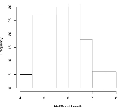
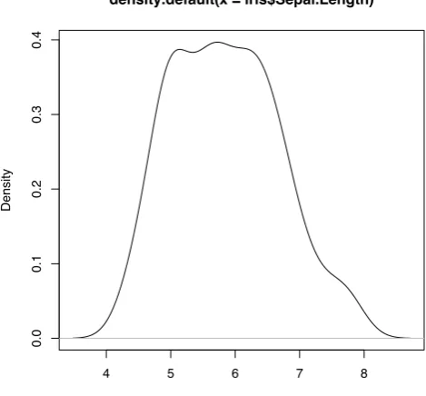
Then we check the variance of Sepal.Lengthwithvar(), and also check its distribution with

histogram and density using functionshist()anddensity().

> var(iris$Sepal.Length)

[1] 0.6856935

> hist(iris$Sepal.Length)

Histogram of iris$Sepal.Length

iris$Sepal.Length

Frequency

4 5 6 7 8

0

5

10

15

20

25

30

(23)

3.2. EXPLORE INDIVIDUAL VARIABLES 13

> plot(density(iris$Sepal.Length))

4 5 6 7 8

0.0

0.1

0.2

0.3

0.4

density.default(x = iris$Sepal.Length)

N = 150 Bandwidth = 0.2736

Density

(24)

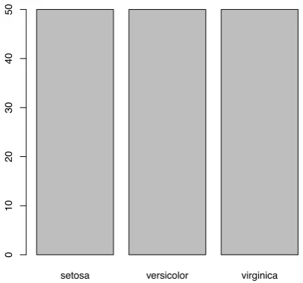
The frequency of factors can be calculated with function table(), and then plotted as a pie

chart withpie()or a bar chart withbarplot().

> table(iris$Species)

setosa versicolor virginica

50 50 50

> pie(table(iris$Species))

setosa

versicolor

virginica

(25)

3.3. EXPLORE MULTIPLE VARIABLES 15

> barplot(table(iris$Species))

0

10

20

30

40

50

Figure 3.4: Bar Chart

3.3 Explore Multiple Variables

After checking the distributions of individual variables, we then investigate the relationships

be-tween two variables. Below we calculate covariance and correlation bebe-tween variables withcov()

andcor().

> cov(iris$Sepal.Length, iris$Petal.Length)

[1] 1.274315

> cov(iris[,1:4])

Sepal.Length Sepal.Width Petal.Length Petal.Width Sepal.Length 0.6856935 -0.0424340 1.2743154 0.5162707 Sepal.Width -0.0424340 0.1899794 -0.3296564 -0.1216394 Petal.Length 1.2743154 -0.3296564 3.1162779 1.2956094 Petal.Width 0.5162707 -0.1216394 1.2956094 0.5810063

> cor(iris$Sepal.Length, iris$Petal.Length)

[1] 0.8717538

> cor(iris[,1:4])

(26)

Next, we compute the stats of Sepal.Lengthof every Specieswithaggregate().

> aggregate(Sepal.Length ~ Species, summary, data=iris)

Species Sepal.Length.Min. Sepal.Length.1st Qu. Sepal.Length.Median

1 setosa 4.300 4.800 5.000

2 versicolor 4.900 5.600 5.900

3 virginica 4.900 6.225 6.500

Sepal.Length.Mean Sepal.Length.3rd Qu. Sepal.Length.Max.

1 5.006 5.200 5.800

2 5.936 6.300 7.000

3 6.588 6.900 7.900

We then use function boxplot() to plot a box plot, also known as box-and-whisker plot, to

show the median, first and third quartile of a distribution (i.e., the 50%, 25% and 75% points in cumulative distribution), and outliers. The bar in the middle is the median. The box shows the interquartile range (IQR), which is the range between the 75% and 25% observation.

> boxplot(Sepal.Length~Species, data=iris)

●

4.5

5.0

5.5

6.0

6.5

7.0

7.5

8.0

Figure 3.5: Boxplot

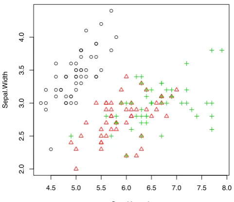
A scatter plot can be drawn for two numeric variables with plot()as below. Using function

(27)

3.3. EXPLORE MULTIPLE VARIABLES 17

and symbols (pch) of points are set toSpecies.

> with(iris, plot(Sepal.Length, Sepal.Width, col=Species, pch=as.numeric(Species)))

●

● ● ●

● ●

●

● ●

●

● ● ●

● ●

● ● ●

●

● ●

●

● ●

●

4.5 5.0 5.5 6.0 6.5 7.0 7.5 8.0

2.0

2.5

3.0

3.5

4.0

Sepal.Length

Sepal.Width

(28)

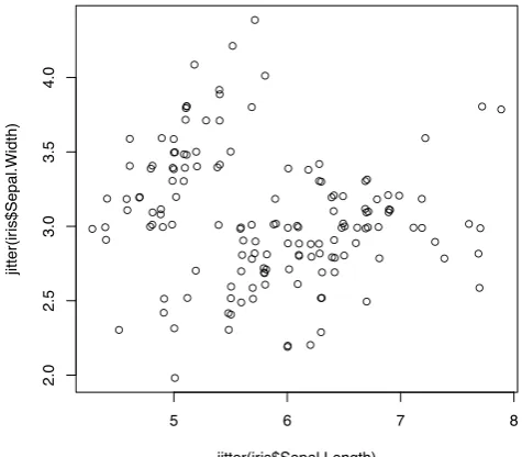
When there are many points, some of them may overlap. We can usejitter()to add a small amount of noise to the data before plotting.

> plot(jitter(iris$Sepal.Length), jitter(iris$Sepal.Width))

●

(29)

3.4. MORE EXPLORATIONS 19

A matrix of scatter plots can be produced with functionpairs().

> pairs(iris)

Sepal.Length

● Sepal.Width

●

Figure 3.8: A Matrix of Scatter Plots

3.4 More Explorations

(30)

A 3D scatter plot can be produced with package scatterplot3d [Ligges and M¨achler, 2003].

> library(scatterplot3d)

> scatterplot3d(iris$Petal.Width, iris$Sepal.Length, iris$Sepal.Width)

0.0 0.5 1.0 1.5 2.0 2.5

Figure 3.9: 3D Scatter plot

Packagergl [Adler and Murdoch, 2012] supports interactive 3D scatter plot withplot3d().

> library(rgl)

> plot3d(iris$Petal.Width, iris$Sepal.Length, iris$Sepal.Width)

A heat map presents a 2D display of a data matrix, which can be generated with heatmap()

(31)

withdist()and then plot it with a heat map.

> distMatrix <- as.matrix(dist(iris[,1:4])) > heatmap(distMatrix)

42 23 14943 39413246 36748316 34 15 45619 21 32 24 25 27 44 17 33 37 49 11 22 47 20 26 31 30 35 10 38541 12 50 28 40829 181

Figure 3.10: Heat Map

A level plot can be produced with function levelplot() in package lattice [Sarkar, 2008].

(32)

rainbow(), which creates a vector of contiguous colors.

> library(lattice)

> levelplot(Petal.Width~Sepal.Length*Sepal.Width, iris, cuts=9,

+ col.regions=grey.colors(10)[10:1])

Sepal.Length

Sepal.Width

2.0 2.5 3.0 3.5 4.0

5 6 7

0.0 0.5 1.0 1.5 2.0 2.5

Figure 3.11: Level Plot

(33)

withcontourplot()in packagelattice.

> filled.contour(volcano, color=terrain.colors, asp=1,

+ plot.axes=contour(volcano, add=T))

100 120 140 160 180 100

100

110 110

110

120

130

140

150 160

160

170

180

190

Figure 3.12: Contour

(34)

generated with functionpersp().

> persp(volcano, theta=25, phi=30, expand=0.5, col="lightblue")

volcano

Y

Z

Figure 3.13: 3D Surface

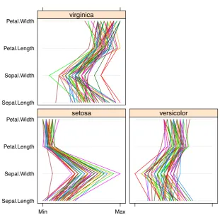
Parallel coordinates provide nice visualization of multiple dimensional data. A parallel

(35)

packagelattice.

> library(MASS)

> parcoord(iris[1:4], col=iris$Species)

Sepal.Length Sepal.Width Petal.Length Petal.Width

(36)

> library(lattice)

> parallelplot(~iris[1:4] | Species, data=iris)

Min Max

setosa versicolor

virginica

Figure 3.15: Parallel Coordinates with Packagelattice

Package ggplot2 [Wickham, 2009] supports complex graphics, which are very useful for

ex-ploring data. A simple example is given below. More examples on that package can be found at

(37)

3.5. SAVE CHARTS INTO FILES 27

> library(ggplot2)

> qplot(Sepal.Length, Sepal.Width, data=iris, facets=Species ~.)

●

Figure 3.16: Scatter Plot with Packageggplot2

3.5 Save Charts into Files

If there are many graphs produced in data exploration, a good practice is to save them into files. R provides a variety of functions for that purpose. Below are examples of saving charts into PDF

and PS files respectively with pdf()and postscript(). Picture files of BMP, JPEG, PNG and

TIFF formats can be generated respectively with bmp(), jpeg(),png() and tiff(). Note that

the files (or graphics devices) need be closed withgraphics.off()or dev.off()after plotting.

> # save as a PDF file > pdf("myPlot.pdf") > x <- 1:50

> plot(x, log(x)) > graphics.off() > #

> # Save as a postscript file > postscript("myPlot2.ps") > x <- -20:20

(38)

(39)

Chapter 4 Decision Trees and Random Forest

This chapter shows how to build predictive models with packagesparty,rpart andrandomForest.

It starts with building decision trees with packageparty and using the built tree for classification,

followed by another way to build decision trees with package rpart. After that, it presents an

example on training a random forest model with packagerandomForest.

4.1 Decision Trees with Package

party

This section shows how to build a decision tree for theirisdata with functionctree()in package

party [Hothorn et al., 2010]. Details of the data can be found in Section 1.3.1. Sepal.Length,

Sepal.Width,Petal.LengthandPetal.Widthare used to predict theSpeciesof flowers. In the

package, functionctree()builds a decision tree, andpredict()makes prediction for new data.

Before modeling, theirisdata is split below into two subsets: training (70%) and test (30%).

The random seed is set to a fixed value below to make the results reproducible.

> str(iris)

$ Species : Factor w/ 3 levels "setosa","versicolor",..: 1 1 1 1 1 1 1 1 1 1 ...

> set.seed(1234)

> ind <- sample(2, nrow(iris), replace=TRUE, prob=c(0.7, 0.3)) > trainData <- iris[ind==1,]

> testData <- iris[ind==2,]

We then load package party, build a decision tree, and check the prediction result. Function

ctree()provides some parameters, such asMinSplit,MinBusket,MaxSurrogateandMaxDepth, to control the training of decision trees. Below we use default settings to build a decision tree.

Ex-amples of setting the above parameters are available in Chapter 13. In the code below,myFormula

specifies thatSpeciesis the target variable and all other variables are independent variables.

> library(party)

> myFormula <- Species ~ Sepal.Length + Sepal.Width + Petal.Length + Petal.Width > iris_ctree <- ctree(myFormula, data=trainData)

> # check the prediction

> table(predict(iris_ctree), trainData$Species)

(40)

setosa 40 0 0

versicolor 0 37 3

virginica 0 1 31

After that, we can have a look at the built tree by printing the rules and plotting the tree.

> print(iris_ctree)

Conditional inference tree with 4 terminal nodes

Response: Species

Inputs: Sepal.Length, Sepal.Width, Petal.Length, Petal.Width Number of observations: 112

1) Petal.Length <= 1.9; criterion = 1, statistic = 104.643 2)* weights = 40

1) Petal.Length > 1.9

3) Petal.Width <= 1.7; criterion = 1, statistic = 48.939 4) Petal.Length <= 4.4; criterion = 0.974, statistic = 7.397

5)* weights = 21 4) Petal.Length > 4.4

6)* weights = 19 3) Petal.Width > 1.7

7)* weights = 32

> plot(iris_ctree)

Petal.Length p < 0.001

1

≤1.9 >1.9

Node 2 (n = 40)

setosa versicolor virginica 0

0.2 0.4 0.6 0.8 1

Petal.Width p < 0.001

3

≤1.7 >1.7

Petal.Length p = 0.026

4

≤4.4 >4.4

Node 5 (n = 21)

0.2 0.4 0.6 0.8 1

Node 6 (n = 19)

0.2 0.4 0.6 0.8 1

Node 7 (n = 32)

0.2 0.4 0.6 0.8 1

(41)

4.1. DECISION TREES WITH PACKAGEPARTY 31

> plot(iris_ctree, type="simple")

Petal.Length p < 0.001

1

≤1.9 >1.9

n = 40 y = (1, 0, 0)

2

Petal.Width p < 0.001

3

≤1.7 >1.7

Petal.Length p = 0.026

4

≤4.4 >4.4

n = 21 y = (0, 1, 0)

5

n = 19 y = (0, 0.842, 0.158)

6

n = 32 y = (0, 0.031, 0.969)

7

Figure 4.2: Decision Tree (Simple Style)

In the above Figure 4.1, the barplot for each leaf node shows the probabilities of an instance falling into the three species. In Figure 4.2, they are shown as “y” in leaf nodes. For example, node 2 is labeled with “n=40, y=(1, 0, 0)”, which means that it contains 40 training instances and all of them belong to the first class “setosa”.

After that, the built tree needs to be tested with test data.

> # predict on test data

> testPred <- predict(iris_ctree, newdata = testData) > table(testPred, testData$Species)

testPred setosa versicolor virginica

setosa 10 0 0

versicolor 0 12 2

virginica 0 0 14

The current version of ctree()(i.e. version 0.9-9995) does not handle missing values well, in

that an instance with a missing value may sometimes go to the left sub-tree and sometimes to the right. This might be caused by surrogate rules.

Another issue is that, when a variable exists in training data and is fed intoctree()but does

not appear in the built decision tree, the test data must also have that variable to make prediction.

Otherwise, a call topredict()would fail. Moreover, if the value levels of a categorical variable in

test data are different from that in training data, it would also fail to make prediction on the test

data. One way to get around the above issue is, after building a decision tree, to callctree()to

build a new decision tree with data containing only those variables existing in the first tree, and to explicitly set the levels of categorical variables in test data to the levels of the corresponding

(42)

4.2 Decision Trees with Package

rpart

Packagerpart [Therneau et al., 2010] is used in this section to build a decision tree on thebodyfat

data (see Section 1.3.2 for details of the data). Functionrpart()is used to build a decision tree,

and the tree with the minimum prediction error is selected. After that, it is applied to new data

to make prediction with functionpredict().

At first, we load thebodyfatdata and have a look at it.

> data("bodyfat", package = "mboost") > dim(bodyfat)

[1] 71 10

> attributes(bodyfat)

$names

[1] "age" "DEXfat" "waistcirc" "hipcirc" "elbowbreadth" [6] "kneebreadth" "anthro3a" "anthro3b" "anthro3c" "anthro4"

$row.names

[1] "47" "48" "49" "50" "51" "52" "53" "54" "55" "56" "57" "58" "59" [14] "60" "61" "62" "63" "64" "65" "66" "67" "68" "69" "70" "71" "72" [27] "73" "74" "75" "76" "77" "78" "79" "80" "81" "82" "83" "84" "85" [40] "86" "87" "88" "89" "90" "91" "92" "93" "94" "95" "96" "97" "98" [53] "99" "100" "101" "102" "103" "104" "105" "106" "107" "108" "109" "110" "111" [66] "112" "113" "114" "115" "116" "117"

$class

[1] "data.frame"

> bodyfat[1:5,]

age DEXfat waistcirc hipcirc elbowbreadth kneebreadth anthro3a anthro3b

47 57 41.68 100.0 112.0 7.1 9.4 4.42 4.95

48 65 43.29 99.5 116.5 6.5 8.9 4.63 5.01

49 59 35.41 96.0 108.5 6.2 8.9 4.12 4.74

50 58 22.79 72.0 96.5 6.1 9.2 4.03 4.48

51 60 36.42 89.5 100.5 7.1 10.0 4.24 4.68

anthro3c anthro4 47 4.50 6.13 48 4.48 6.37 49 4.60 5.82 50 3.91 5.66 51 4.15 5.91

Next, the data is split into training and test subsets, and a decision tree is built on the training data.

> set.seed(1234)

> ind <- sample(2, nrow(bodyfat), replace=TRUE, prob=c(0.7, 0.3)) > bodyfat.train <- bodyfat[ind==1,]

> bodyfat.test <- bodyfat[ind==2,] > # train a decision tree

> library(rpart)

> myFormula <- DEXfat ~ age + waistcirc + hipcirc + elbowbreadth + kneebreadth > bodyfat_rpart <- rpart(myFormula, data = bodyfat.train,

+ control = rpart.control(minsplit = 10))

(43)

4.2. DECISION TREES WITH PACKAGERPART 33

$names

[1] "frame" "where" "call" [4] "terms" "cptable" "method" [7] "parms" "control" "functions"

[10] "numresp" "splits" "variable.importance" [13] "y" "ordered"

$xlevels named list()

$class [1] "rpart"

> print(bodyfat_rpart$cptable)

CP nsplit rel error xerror xstd 1 0.67272638 0 1.00000000 1.0194546 0.18724382 2 0.09390665 1 0.32727362 0.4415438 0.10853044 3 0.06037503 2 0.23336696 0.4271241 0.09362895 4 0.03420446 3 0.17299193 0.3842206 0.09030539 5 0.01708278 4 0.13878747 0.3038187 0.07295556 6 0.01695763 5 0.12170469 0.2739808 0.06599642 7 0.01007079 6 0.10474706 0.2693702 0.06613618 8 0.01000000 7 0.09467627 0.2695358 0.06620732

> print(bodyfat_rpart)

n= 56

node), split, n, deviance, yval * denotes terminal node

1) root 56 7265.0290000 30.94589

2) waistcirc< 88.4 31 960.5381000 22.55645 4) hipcirc< 96.25 14 222.2648000 18.41143

8) age< 60.5 9 66.8809600 16.19222 * 9) age>=60.5 5 31.2769200 22.40600 * 5) hipcirc>=96.25 17 299.6470000 25.97000

10) waistcirc< 77.75 6 30.7345500 22.32500 * 11) waistcirc>=77.75 11 145.7148000 27.95818

22) hipcirc< 99.5 3 0.2568667 23.74667 * 23) hipcirc>=99.5 8 72.2933500 29.53750 * 3) waistcirc>=88.4 25 1417.1140000 41.34880

6) waistcirc< 104.75 18 330.5792000 38.09111 12) hipcirc< 109.9 9 68.9996200 34.37556 * 13) hipcirc>=109.9 9 13.0832000 41.80667 * 7) waistcirc>=104.75 7 404.3004000 49.72571 *

(44)

> plot(bodyfat_rpart)

> text(bodyfat_rpart, use.n=T)

| waistcirc< 88.4

hipcirc< 96.25

age< 60.5 waistcirc< 77.75

hipcirc< 99.5

waistcirc< 104.8

hipcirc< 109.9 16.19

n=9

22.41

n=5 _22.32

n=6 23.75_n=3 29.54_n=8 34.38_n=9 41.81_n=9

49.73 n=7

Figure 4.3: Decision Tree with Packagerpart

(45)

4.2. DECISION TREES WITH PACKAGERPART 35

> opt <- which.min(bodyfat_rpart$cptable[,"xerror"]) > cp <- bodyfat_rpart$cptable[opt, "CP"]

> bodyfat_prune <- prune(bodyfat_rpart, cp = cp) > print(bodyfat_prune)

n= 56

node), split, n, deviance, yval * denotes terminal node

1) root 56 7265.02900 30.94589

2) waistcirc< 88.4 31 960.53810 22.55645 4) hipcirc< 96.25 14 222.26480 18.41143

8) age< 60.5 9 66.88096 16.19222 * 9) age>=60.5 5 31.27692 22.40600 * 5) hipcirc>=96.25 17 299.64700 25.97000

10) waistcirc< 77.75 6 30.73455 22.32500 * 11) waistcirc>=77.75 11 145.71480 27.95818 * 3) waistcirc>=88.4 25 1417.11400 41.34880

6) waistcirc< 104.75 18 330.57920 38.09111 12) hipcirc< 109.9 9 68.99962 34.37556 * 13) hipcirc>=109.9 9 13.08320 41.80667 * 7) waistcirc>=104.75 7 404.30040 49.72571 *

> plot(bodyfat_prune)

> text(bodyfat_prune, use.n=T)

| waistcirc< 88.4

hipcirc< 96.25

age< 60.5 waistcirc< 77.75

waistcirc< 104.8

hipcirc< 109.9 16.19

n=9

22.41 n=5

22.32 n=6

27.96

n=11 34.38

n=9

41.81 n=9

49.73 n=7

Figure 4.4: Selected Decision Tree

After that, the selected tree is used to make prediction and the predicted values are compared

with actual labels. In the code below, functionabline()draws a diagonal line. The predictions

(46)

> DEXfat_pred <- predict(bodyfat_prune, newdata=bodyfat.test) > xlim <- range(bodyfat$DEXfat)

> plot(DEXfat_pred ~ DEXfat, data=bodyfat.test, xlab="Observed",

+ ylab="Predicted", ylim=xlim, xlim=xlim)

> abline(a=0, b=1)

●

● ●

●

● ●

●

● ●

●

● ●

10 20 30 40 50 60

10

20

30

40

50

60

Observed

Predicted

Figure 4.5: Prediction Result

4.3 Random Forest

Package randomForest [Liaw and Wiener, 2002] is used below to build a predictive model for

theirisdata (see Section 1.3.1 for details of the data). There are two limitations with function

randomForest(). First, it cannot handle data with missing values, and users have to impute data before feeding them into the function. Second, there is a limit of 32 to the maximum number of levels of each categorical attribute. Attributes with more than 32 levels have to be transformed

first before usingrandomForest().

An alternative way to build a random forest is to use function cforest()from packageparty,

which is not limited to the above maximum levels. However, generally speaking, categorical variables with more levels will make it require more memory and take longer time to build a random forest.

Again, the irisdata is first split into two subsets: training (70%) and test (30%).

> ind <- sample(2, nrow(iris), replace=TRUE, prob=c(0.7, 0.3)) > trainData <- iris[ind==1,]

> testData <- iris[ind==2,]

Then we load packagerandomForestand train a random forest. In the code below, the formula

is set to “Species ∼ _.”, which means to predict_Specieswith all other variables in the data.

> library(randomForest)

(47)

4.3. RANDOM FOREST 37

setosa 36 0 0

versicolor 0 31 1

virginica 0 1 35

> print(rf)

Call:

randomForest(formula = Species ~ ., data = trainData, ntree = 100, proximity = TRUE) Type of random forest: classification

Number of trees: 100 No. of variables tried at each split: 2

OOB estimate of error rate: 1.92% Confusion matrix:

setosa versicolor virginica class.error

setosa 36 0 0 0.00000000

versicolor 0 31 1 0.03125000

virginica 0 1 35 0.02777778

> attributes(rf)

$names

[1] "call" "type" "predicted" "err.rate" [5] "confusion" "votes" "oob.times" "classes" [9] "importance" "importanceSD" "localImportance" "proximity" [13] "ntree" "mtry" "forest" "y"

[17] "test" "inbag" "terms"

$class

(48)

After that, we plot the error rates with various number of trees.

> plot(rf)

0 20 40 60 80 100

0.00

0.05

0.10

0.15

0.20

rf

trees

Error

Figure 4.6: Error Rate of Random Forest

(49)

4.3. RANDOM FOREST 39

> importance(rf)

MeanDecreaseGini Sepal.Length 6.485090 Sepal.Width 1.380624 Petal.Length 32.498074 Petal.Width 28.250058

> varImpPlot(rf)

Sepal.Width Sepal.Length Petal.Width Petal.Length

● ●

0 5 10 15 20 25 30

rf

MeanDecreaseGini

Figure 4.7: Variable Importance

Finally, the built random forest is tested on test data, and the result is checked with functions

(50)

means correct classification.

> irisPred <- predict(rf, newdata=testData) > table(irisPred, testData$Species)

irisPred setosa versicolor virginica

setosa 14 0 0

versicolor 0 17 3

virginica 0 1 11

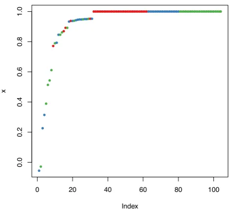
> plot(margin(rf, testData$Species))

●

● ●

● ● ●

●

●●

● ●●●

● ●●

●●●●●●●●●●●●●●

●●●●●●●●●●●●●●●●●●●●●●●●●●●●●●●●●●●●●●●●●●●●●●●●●●●●●●●●●●●●●●●●●●●●●●●●●

0 20 40 60 80 100

0.0

0.2

0.4

0.6

0.8

1.0

Index

x

(51)

Chapter 5 Regression

Regression is to build a function of independent variables (also known aspredictors) to predict

a dependent variable (also called response). For example, banks assess the risk of home-loan applicants based on their age, income, expenses, occupation, number of dependents, total credit limit, etc.

This chapter introduces basic concepts and presents examples of various regression techniques. At first, it shows an example on building a linear regression model to predict CPI data. After that, it introduces logistic regression. The generalized linear model (GLM) is then presented, followed by a brief introduction of non-linear regression.

A collection of some helpful R functions for regression analysis is available as a reference card onR Functions for Regression Analysis 1_.

5.1 Linear Regression

Linear regression is to predict response with a linear function of predictors as follows:

y=c0+c1x1+c2x2+· · ·+ckxk,

wherex1, x2,· · ·, xk are predictors andy is the response to predict.

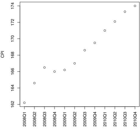
Linear regression is demonstrated below with functionlm()on the Australian CPI (Consumer

Price Index) data, which are quarterly CPIs from 2008 to 20102_.

At first, the data is created and plotted. In the code below, an x-axis is added manually with

functionaxis(), where las=3makes text vertical.

1

http://cran.r-project.org/doc/contrib/Ricci-refcard-regression.pdf 2_{From Australian Bureau of Statistics}

<http://www.abs.gov.au>

(52)

> year <- rep(2008:2010, each=4) > quarter <- rep(1:4, 3)

> cpi <- c(162.2, 164.6, 166.5, 166.0,

+ 166.2, 167.0, 168.6, 169.5,

+ 171.0, 172.1, 173.3, 174.0)

> plot(cpi, xaxt="n", ylab="CPI", xlab="") > # draw x-axis

> axis(1, labels=paste(year,quarter,sep="Q"), at=1:12, las=3)

● ●

●

● ● ●

● ●

162

164

166

168

170

172

174

CPI

2008Q1 2008Q2 2008Q3 2008Q4 2009Q1 2009Q2 2009Q3 2009Q4 2010Q1 2010Q2 2010Q3 2010Q4

Figure 5.1: Australian CPIs in Year 2008 to 2010

We then check the correlation betweenCPIand the other variables,yearandquarter.

> cor(year,cpi)

[1] 0.9096316

> cor(quarter,cpi)

[1] 0.3738028

Then a linear regression model is built with function lm()on the above data, usingyearand

quarteras predictors andCPIas response. > fit <- lm(cpi ~ year + quarter) > fit

Call:

lm(formula = cpi ~ year + quarter)

Coefficients:

(Intercept) year quarter

(53)

5.1. LINEAR REGRESSION 43

With the above linear model, CPI is calculated as

cpi =c0+c1∗year +c2∗quarter,

where c0, c1 and c2 are coefficients from model fit. Therefore, the CPIs in 2011 can be get as

follows. An easier way for this is using functionpredict(), which will be demonstrated at the

end of this subsection.

> (cpi2011 <- fit$coefficients[[1]] + fit$coefficients[[2]]*2011 +

+ fit$coefficients[[3]]*(1:4))

[1] 174.4417 175.6083 176.7750 177.9417

More details of the model can be obtained with the code below.

> attributes(fit)

$names

[1] "coefficients" "residuals" "effects" "rank"

[5] "fitted.values" "assign" "qr" "df.residual" [9] "xlevels" "call" "terms" "model"

$class [1] "lm"

> fit$coefficients

(Intercept) year quarter -7644.487500 3.887500 1.166667

The differences between observed values and fitted values can be obtained with function

resid-uals().

> # differences between observed values and fitted values > residuals(fit)

1 2 3 4 5 6

-0.57916667 0.65416667 1.38750000 -0.27916667 -0.46666667 -0.83333333

7 8 9 10 11 12

-0.40000000 -0.66666667 0.44583333 0.37916667 0.41250000 -0.05416667

> summary(fit)

Call:

lm(formula = cpi ~ year + quarter)

Residuals:

Min 1Q Median 3Q Max

-0.8333 -0.4948 -0.1667 0.4208 1.3875

Coefficients:

Estimate Std. Error t value Pr(>|t|) (Intercept) -7644.4875 518.6543 -14.739 1.31e-07 *** year 3.8875 0.2582 15.058 1.09e-07 *** quarter 1.1667 0.1885 6.188 0.000161 ***

---Signif. codes: 0 ´S***ˇS 0.001 ´S**ˇS 0.01 ´S*ˇS 0.05 ´S.ˇS 0.1 ´S ˇS 1

Residual standard error: 0.7302 on 9 degrees of freedom

(54)

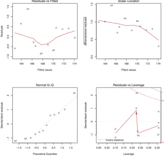
We then plot the fitted model as below.

> plot(fit)

164 166 168 170 172 174

−

Fitted values

Residuals Residuals vs Fitted

3

Theoretical Quantiles

Standardiz

ed residuals

Normal Q−Q

3

6 8

164 166 168 170 172 174

0.0

0.5

1.0

1.5

Fitted values

Standardized residuals

● ● Scale−Location

3

6 8

0.00 0.05 0.10 0.15 0.20 0.25 0.30 0.35

−

ed residuals

●

Cook's distance

0.5 0.5 1

Residuals vs Leverage

3

1 8

Figure 5.2: Prediction with Linear Regression Model - 1

We can also plot the model in a 3D plot as below, where function scatterplot3d() creates

a 3D scatter plot and plane3d() draws the fitted plane. Parameterlabspecifies the number of

(55)

5.1. LINEAR REGRESSION 45

> library(scatterplot3d)

> s3d <- scatterplot3d(year, quarter, cpi, highlight.3d=T, type="h", lab=c(2,3)) > s3d$plane3d(fit)

2008160 2009 2010

165

170

175

1 2

3 4

year

quar

ter

cpi

●

Figure 5.3: A 3D Plot of the Fitted Model

(56)

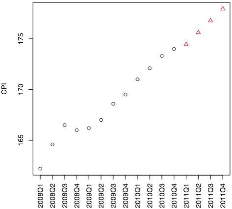
> data2011 <- data.frame(year=2011, quarter=1:4) > cpi2011 <- predict(fit, newdata=data2011) > style <- c(rep(1,12), rep(2,4))

> plot(c(cpi, cpi2011), xaxt="n", ylab="CPI", xlab="", pch=style, col=style) > axis(1, at=1:16, las=3,

+ labels=c(paste(year,quarter,sep="Q"), "2011Q1", "2011Q2", "2011Q3", "2011Q4"))

● ●

● ● ●

● ●

●

165

170

175

CPI

2008Q1 2008Q2 2008Q3 2008Q4 2009Q1 2009Q2 2009Q3 2009Q4 2010Q1 2010Q2 2010Q3 2010Q4 2011Q1 2011Q2 2011Q3 2011Q4

Figure 5.4: Prediction of CPIs in 2011 with Linear Regression Model

5.2 Logistic Regression

Logistic regression is used to predict the probability of occurrence of an event by fitting data to a logistic curve. A logistic regression model is built as the following equation:

logit(y) =c0+c1x1+c2x2+· · ·+ckxk,

wherex1, x2,· · ·, xk are predictors,y is a response to predict, andlogit(y) =ln(₁y

−y). The above

equation can also be written as

y= 1

1 +e−(c0+c1x1+c2x2+_···+ckxk).

Logistic regression can be built with functionglm()by settingfamilytobinomial(link="logit").

Detailed introductions on logistic regression can be found at the following links.

R Data Analysis Examples - Logit Regression

http://www.ats.ucla.edu/stat/r/dae/logit.htm

Logistic Regression (with R)

(57)

5.3. GENERALIZED LINEAR REGRESSION 47

5.3 Generalized Linear Regression

The generalized linear model (GLM) generalizes linear regression by allowing the linear model to be related to the response variable via a link function and allowing the magnitude of the variance of each measurement to be a function of its predicted value. It unifies various other statistical

models, including linear regression, logistic regression and Poisson regression. Function glm()

is used to fit generalized linear models, specified by giving a symbolic description of the linear predictor and a description of the error distribution.

A generalized linear model is built below with glm() on the bodyfatdata (see Section 1.3.2

for details of the data).

> data("bodyfat", package="mboost")

> myFormula <- DEXfat ~ age + waistcirc + hipcirc + elbowbreadth + kneebreadth > bodyfat.glm <- glm(myFormula, family = gaussian("log"), data = bodyfat) > summary(bodyfat.glm)

Call:

glm(formula = myFormula, family = gaussian("log"), data = bodyfat)

Deviance Residuals:

Min 1Q Median 3Q Max

-11.5688 -3.0065 0.1266 2.8310 10.0966

Coefficients:

Estimate Std. Error t value Pr(>|t|) (Intercept) 0.734293 0.308949 2.377 0.02042 * age 0.002129 0.001446 1.473 0.14560 waistcirc 0.010489 0.002479 4.231 7.44e-05 *** hipcirc 0.009702 0.003231 3.003 0.00379 ** elbowbreadth 0.002355 0.045686 0.052 0.95905 kneebreadth 0.063188 0.028193 2.241 0.02843 *

---Signif. codes: 0 ´S***ˇS 0.001 ´S**ˇS 0.01 ´S*ˇS 0.05 ´S.ˇS 0.1 ´S ˇS 1

(Dispersion parameter for gaussian family taken to be 20.31433)

Null deviance: 8536.0 on 70 degrees of freedom Residual deviance: 1320.4 on 65 degrees of freedom AIC: 423.02

Number of Fisher Scoring iterations: 5

> pred <- predict(bodyfat.glm, type="response")

In the code above,type indicates the type of prediction required. The default is on the scale of

(58)

> plot(bodyfat$DEXfat, pred, xlab="Observed Values", ylab="Predicted Values") > abline(a=0, b=1)

●●

●

● ●

●

● ●

●

● ●

●

● ●

●

● ●

●

● ●

●

● ●

●

● ●

●

● ●

●

● ● ●

● ●

●

10 20 30 40 50 60

20

30

40

50

Observed Values

Predicted V

alues

Figure 5.5: Prediction with Generalized Linear Regression Model

In the above code, if family=gaussian("identity")is used, the built model would be

sim-ilar to linear regression. One can also make it a logistic regression by setting family to

bino-mial("logit").

5.4 Non-linear Regression

While linear regression is to find the line that comes closest to data, non-linear regression is to

fit a curve through data. Functionnls()provides nonlinear regression. Examples of nls() can be

(59)

Chapter 6 Clustering

This chapter presents examples of various clustering techniques in R, includingk-means clustering,

k-medoids clustering, hierarchical clustering and density-based clustering. The first two sections

demonstrate how to use thek-means andk-medoids algorithms to cluster theirisdata. The third

section shows an example on hierarchical clustering on the same data. The last section describes the idea of density-based clustering and the DBSCAN algorithm, and shows how to cluster with DBSCAN and then label new data with the clustering model. For readers who are not familiar with clustering, introductions of various clustering techniques can be found in [Zhao et al., 2009a] and [Jain et al., 1999].

6.1 The k-Means Clustering

This section shows k-means clustering of iris data (see Section 1.3.1 for details of the data).

At first, we remove species from the data to cluster. After that, we apply functionkmeans()to

iris2, and store the clustering result in kmeans.result. The cluster number is set to 3 in the code below.

> iris2 <- iris

> iris2$Species <- NULL

> (kmeans.result <- kmeans(iris2, 3))

K-means clustering with 3 clusters of sizes 38, 50, 62

Cluster means:

Sepal.Length Sepal.Width Petal.Length Petal.Width 1 6.850000 3.073684 5.742105 2.071053 2 5.006000 3.428000 1.462000 0.246000 3 5.901613 2.748387 4.393548 1.433871

Clustering vector:

[1] 2 2 2 2 2 2 2 2 2 2 2 2 2 2 2 2 2 2 2 2 2 2 2 2 2 2 2 2 2 2 2 2 2 2 2 2 2 2 2 [40] 2 2 2 2 2 2 2 2 2 2 2 3 3 1 3 3 3 3 3 3 3 3 3 3 3 3 3 3 3 3 3 3 3 3 3 3 3 3 1 [79] 3 3 3 3 3 3 3 3 3 3 3 3 3 3 3 3 3 3 3 3 3 3 1 3 1 1 1 1 3 1 1 1 1 1 1 3 3 1 1 [118] 1 1 3 1 3 1 3 1 1 3 3 1 1 1 1 1 3 1 1 1 1 3 1 1 1 3 1 1 1 3 1 1 3

Within cluster sum of squares by cluster: [1] 23.87947 15.15100 39.82097

(between_SS / total_SS = 88.4 %)

Available components:

(60)

[1] "cluster" "centers" "totss" "withinss" "tot.withinss" [6] "betweenss" "size"

The clustering result is then compared with the class label (Species) to check whether similar

objects are grouped together.

> table(iris$Species, kmeans.result$cluster)

1 2 3 setosa 0 50 0 versicolor 2 0 48 virginica 36 0 14

The above result shows that cluster “setosa” can be easily separated from the other clusters, and that clusters “versicolor” and “virginica” are to a small degree overlapped with each other.

Next, the clusters and their centers are plotted (see Figure 6.1). Note that there are four dimensions in the data and that only the first two dimensions are used to draw the plot below. Some black points close to the green center (asterisk) are actually closer to the black center in the four dimensional space. We also need to be aware that the results of k-means clustering may vary from run to run, due to random selection of initial cluster centers.

> plot(iris2[c("Sepal.Length", "Sepal.Width")], col = kmeans.result$cluster) > # plot cluster centers

> points(kmeans.result$centers[,c("Sepal.Length", "Sepal.Width")], col = 1:3,

+ pch = 8, cex=2)

Figure 6.1: Results of k-Means Clustering

(61)

6.2. THE K-MEDOIDS CLUSTERING 51

6.2 The k-Medoids Clustering

This sections shows k-medoids clustering with functionspam()andpamk(). The k-medoids

clus-tering is very similar to k-means, and the major difference between them is that: while a cluster

is represented with its center in the k-means algorithm, it is represented with the object closest to the center of the cluster in the k-medoids clustering. The k-medoids clustering is more robust than k-means in presence of outliers. PAM (Partitioning Around Medoids) is a classic algorithm for

k-medoids clustering. While the PAM algorithm is inefficient for clustering large data, the CLARA

algorithm is an enhanced technique of PAM by drawing multiple samples of data, applying PAM on each sample and then returning the best clustering. It performs better than PAM on larger

data. Functionspam()andclara()in packagecluster [Maechler et al., 2012] are respectively

im-plementations of PAM and CLARA in R. For both algorithms, a user has to specifyk, the number

of clusters to find. As an enhanced version ofpam(), functionpamk()in packagefpc[Hennig, 2010]

does not require a user to choosek. Instead, it calls the functionpam()orclara()to perform a

partitioning around medoids clustering with the number of clusters estimated by optimum average silhouette width.

With the code below, we demonstrate how to find clusters withpam() andpamk().

> library(fpc)

> pamk.result <- pamk(iris2) > # number of clusters > pamk.result$nc

[1] 2

> # check clustering against actual species

> table(pamk.result$pamobject$clustering, iris$Species)

1 50 1 0

R and Data Mining: Examples and Case Studies