IDENTIFICATION OF PROMINENT SPATIO-TEMPORAL SIGNALS IN GRACE
DERIVED TERRESTRIAL WATER STORAGE FOR INDIA
Chandan Banerjeea and D Nagesh Kumara,b
a
Department of Civil Engineering, Indian Institute of Science, Bangalore, India – (chandanb, nagesh)@civil.iisc.ernet.in b
Centre for Earth Sciences, Indian Institute of Science, Bangalore, India
KEY WORDS: GRACE, Terrestrial Water Storage, PCA, ICA, Seasonality, Trend
ABSTRACT:
Fresh water is a necessity of the human civilization. But with the increasing global population, the quantity and quality of available fresh water is getting compromised. To mitigate this subliminal problem, it is essential to enhance our level of understanding abou t the dynamics of global and regional fresh water resources which include surface and ground water reserves. With development in remote sensing technology, traditional and much localized in-situ observations are augmented with satellite data to get a holistic picture of the terrestrial water resources. For this reason, Gravity Recovery And Climate Experiment (GRACE) satellite mission was jointly implemented by NASA and German Aerospace Research Agency – DLR to map the variation of gravitational potential, which after removing atmospheric and oceanic effects is majorly caused by changes in Terrestrial Water Storage (TWS). India also faces the challenge of rejuvenating the fast deteriorating and exhausting water resources due to the rapid urbanization . In the present study we try to identify physically meaningful major spatial and temporal patterns or signals of changes in TWS for India. TWS data set over India for a period of 90 months, from June 2003 to December 2010 is use to isolate spatial and temporal signals using Principal Component Analysis (PCA), an extensively used method in meteorological studies. To achieve better disintegration of the data into more physically meaningful components we use a blind signal separation technique, Independent Component Analysis (ICA). pumping of ground water, constantly polluted surface water reserves, improper use and storage of rainfall often resulting in floods and droughts. A UNICEF report in 2013 also said that the time bomb of increasing water pollution is ticking.
Tackling a problem of this dimension requires effective management which in turn requires efficient monitoring of water resources. In an era of advanced satellite technology, in-situ measurements are augmented by remotely sensed observations. One such technique is Gravity Recovery and Climate Experiment (GRACE), a twin satellite system that has been measuring the gravity field of the Earth (Tapley et al., 2004a,b) for more than a decade now.
GRACE has helped identify many problems and the respective sources which were not detectable or explainable before. Ramillien et al. (2006) used GRACE data to estimate time series of basin scale regional evapotranspiration rate and associated uncertainties. Sun (2013) tried to downscale GRACE data for prediction of ground water level changes. Water storage interannual variability over West Africa was determined by GRACE data by Grippa et al. (2011). Reager et al. (2009) tried to quantify the global terrestrial water storage capacity and flood potential. Alsdorf et al. (2010) used GRACE data along with other satellite observations to quantify the amounts of water filling and draining from the mainstem Amazon floodplain.
Very few studies have used GRACE data to access the water problems in India. Rodell et al. (2009) and Tiwari et al. (2009) unraveled the alarming rate of depletion of ground water in the north western states of India. They clearly stated that if the problem is not controlled immediately, it may result in acute shortage of water in this region. GRACE data also provided insight into the water storage dynamics of Himalayan and Tibetan region (Moiwo et al. 2011), evapotranspiration over the Ganga river basin (Syed at al. 2014) and seasonality and trend in groundwater storage associated with intensive groundwater abstraction in the Bengal basin of Bangladesh (Shamsudduha et al. 2012). There is a scope to explore the valuable and unprecedented GRACE data to estimate the major water reservoirs in India, their spatial and temporal dynamics and try to solve major water crisis. In the present study we try to understand the dynamics of the Terrestrial Water Storage (TWS) by isolating prominent and physically meaningful spatio-temporal signals.
overcome this problem, a blind signal separation technique is generally used called the Independent Component Analysis (Hyvärinen, 1999a,b; Hyvärinen & Oja, 2000). In this study, ICA is shown as an extension of PCA, i.e. a linear transformation of principal components (PCs) where the independent components (ICs) derived are statistically independent and not merely orthogonal. Statistical independence is ensured by using the fourth order statistic or cumulant also known as kurtosis instead of second order statistic i.e. variance-covariance. Forootan and Kusche (2012) showed that ICA works well as compared to PCA for isolation of prominent spatial and temporal patterns of GRACE TWS. Consequently ICA has been used for extracting dominant patterns of TWS changes over Australia (Forootan et al. 2012), Iran (Forootan et al. 2014) and in Nile basin (Awange et al. 2014). In this paper we use both PCA and ICA for spatio-temporal signal separation of TWS changes. In the subsequent sections we discuss about the data used for the study, details about the PCA and ICA techniques, results of the analysis and finally the outcomes.
2. DATA AND METHODS
2.1 Data
In the present work we have used the Global data set publicly available at the Jet Propulsion Laboratory’s TELLUS website (available at http://grace.jpl.nasa.gov). This is a third level GRACE data set represented in terms of centimeters of equivalent water height at a spatial resolution of 1ox1o and a temporal resolution of a month with some data gaps. The second level data set of GRACE is a set of spherical harmonic coefficients. The TELLUS data set is derived from RL05 removes systematic errors manifested as north-south-oriented stripes in maps of GRACE TWS. The second filter is a Gaussian averaging filter that reduces random errors in higher degree spherical harmonic coefficients not removed by the previous filtering operation (Swenson and Wahr, 2006). Out of the three data sets derived from three different sources we use the CSR data for a period of 90 months starting from July 2003 to December 2010. An areal extent of the data extracted for the study covers 65o E to 90o E and 37o N to 4o N.
2.2 Principal Component Analysis
PCA is a linear transformation of the original data to derive a set of orthogonal vectors that spans the same space and hence forms an orthogonal basis of the vector space. The principal components of a multivariate set of data are computed from the eigenvalues and eigenvectors of either the sample correlation or sample covariance matrix. Let us define a data matrix X ' of dimension n x p where p are the grid-points and n is the sampling dimension, i.e., the number of months of record. Each row contains all the grid points representing a particular month and each column contains a time series of a particular grid. The matrix X' is then centered by subtracting the temporal means of each time series respectively to obtain a matrix X. We use singular value decomposition to obtain the PCs (temporal modes) and empirical orthogonal functions or EOFs (spatial patterns). The decomposition is done according to the following equation.
T
X P E (1)
where P contains the PCs
contains the singular values in descending order E contains the EOFs
Out of the n spatial and temporal components extracted using PCA analysis, we retain only j of them such that it explains most of the variance of the data. Hence eq. (1) can be rewritten as
T
j j j
X P E
(2)
2.3 Independent Component Analysis
ICA is a computationally efficient blind signal separation technique explored as a tool in many disciplines of science and engineering. A general mathematical model used to represent ICA can be written as follows.
x As
(3)
where x is a vector representing observed signals s is a vector representing source signals A is the mixing matrix
The two major assumptions of ICA are (i) the signal sources are statistically independent and (ii) the observations have Gaussian distribution. Here we define measure of non-gaussianity by kurtosis of a time series as
4 kurtosis greater than 0.5 indicates a non-Gaussian distribution (Westra et al., 2007). PCA is considered as a pre-processing of ICA, where the first few orthogonal components are analyzed to obtain independent components. In this study ICA is considered as an extension of PCA, as considered by Forootan and Kusche, 2011. The leading PCs and EOFs are rotated to independence to obtain temporal and spatial independent components respectively. This can be represented as follows.
T T
j j j j j
X P R R E (5)
Figure 1 Variance and cumulative percentage of variance described by the first 20 principal components
3. RESULTS
We start our analysis with the construction of the centered data matrix X. Principal component analysis is performed by solving the eigenvalue problem, which gives the eigenvectors or principal components and the associated eigenvalues or variances. The principal components are ordered in decreasing order of variance. Figure 1 show the variance associated with the first 20 PCs out of a total of 90. We retain the first 6 PCs which represent 34.5, 13.2, 9.3, 8.1, 4.5 and 3.1 percent of variance with a total of 72.9 percent.
Figure 2 and 3 shows the temporal and spatial components or the PCs and EOFs respectively. The PCs are represented in normalized form and the normalized EOFs are multiplied to the respective variance and then plotted as temporal patterns. The first component which describes the maximum variability can be interpreted as the seasonal component, with a cycle of one year. The spatial pattern shows that the areas showing most of the seasonality cover the major river basins in India. Most prominent seasonal variation is observed in the lower reaches of river Ganga, where the seasonal variation peaks around the
This temporal pattern is similar for most of the river basins in India which enjoys the Indian monsoon as a major source of water. As there are many different sources of water and varied characteristics of a river basin which dictates its response, the seasonal pattern has varying intensity across space. The northern most parts show an opposite seasonality peaking in December and reaching the minimum around August. It can also be observed from the first PC that the coastal regions show almost no seasonal variation of water storage. The second PC represents a trend and seasonality in some sense but it is not very obvious and interpretable. Rest of the PC’s, which describe very less variability, are noisy and hence not at all interpretable.
As the next step of analysis, we first find the kurtosis of the grid-point time series derived according to Eq. 2 shows. We find that 63% of the grid points have absolute value of kurtosis more than 0.5 and hence exhibit a non-Gaussian distribution. Now we perform independent component analysis, using the temporal and spatial components obtained from PCA as whitened observations. First we perform temporal ICA and then find its projection to get the corresponding spatial pattern. Although not very significant but an ambiguity exits in magnitude and scaling of ICA, hence the magnitudes represented in the figures do not have physical meaning in itself, but has comparative implication. Figure 4 and 5 shows the result of temporal ICA. The very first observation is that the ICA works better than PCA in extracting the prominent patterns. IC1 shows the dominant signal of seasonality. Figure 2 Performance of PCA in extracting dominant temporal
patterns. First six principal components or temporal patterns in decreasing order of magnitude of variance associated
Figure 4 Performance of temporal ICA. First six dominant temporal patterns in decreasing order of magnitude of variance
associated
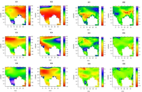
Figure 5 Performance of temporal ICA. First six dominant spatial patterns associated with the temporal modes of Fig. 4
The spatial pattern shows that this seasonal component is predominant in north eastern part of India peaking in around August. There is also an opposite behavior notices in peninsular India. IC2 also indicates another seasonal component which peaks in the month of July and is a significant signature of almost whole of India. IC3 is some sort a noisy trend, which is predominant in the north western part of India. A very similar observation was done by Rodell et al. (2009) and Tiwari et al. (2009). The other components are majorly noisy and it is difficult to associate any physical meaning with them.
Next we perform spatial ICA using the EOFs as the whitened observations. The results show more spatially localized patterns and 4 clearly distinguishable temporal modes. IC1 and IC2 are dominant features of the north eastern parts of India and lower reaches of Ganga basin respectively, where TWS peaks around the month of August, attributable to the Indian monsoon. An opposite behavior, featuring lowest TWS in August is observed in the central and southern parts and western parts for IC1 and IC2 respectively. IC3 shows a significant decreasing trend in northern and north western India, whereas an increasing trend in peninsular India.
CONCLUSION
We have successfully implemented PCA and ICA techniques for the extraction of prominent spatial and temporal patterns of GRACE TWS over India. A major observation is the seasonality of TWS over large parts of the country comfortably attributable to the Indian monsoon which is one of the major source of water for all purposes, ranging from agricultural to domestic, industrial to commercial. Another dominant feature ICA has captured unlike PCA is the decreasing trend of TWS in the northern and north-western parts of the country. Rodell et al. (2009) have attributed this loss to the alarmingly fast rate of depletion of ground water in these areas. Also, the coastal areas show almost no change in TWS throughout the whole study period of 90 months. More detailed reasons of the spatio-temporal patterns of TWS will be evident only when compared with other observations like precipitation and evapotranspiration fluxes, soil moisture and surface water storage changes.
ACKNOWLEDGEMENT
GRACE land data were processed by Sean Swenson, supported by the NASA MEaSUREs Program, and are available at http://grace.jpl.nasa.gov.
REFERENCES
Alsdorf, D., Paul Bates, S. C. H., and Melack, J., 2010. Seasonal water storage on the Amazon floodplain measured from satellites. Remote Sensing of Environment 114, 2448– 2456.
Awange, J.L., Fleming, K.M., Kuhn, M., Featherstone, W.E., Heck, B. and Anjasmara, I., 2011. On the suitability of the 4°×4° GRACE mascon solutions for remote sensing Australian hydrology. Remote Sensing of Environment 115, 864–875. Awange, J.L., Forootan, E., Kuhn, M., Kusche, J., and Heck, B., 2014. Water storage changes and climate variability within the Nile Basin between 2002 and 2011, Advances in Water Resources 73, 1–15.
Forootan, E. and Kusche, J., 2012. Separation of global time-variable gravity signals into maximally independent components. J Geod 86:477–497 DOI 10.1007/s00190-011-0532-5.
Forootan, E., Awange, J.L., Kusche, J., Heck, B., and Eicker, A., 2012. Independent patterns of water mass anomalies over Australia from satellite data and models. Remote Sensing of Environment 124, 427–443.
Forootan, E., Rietbroek, R., Kusche, J., Sharifi, M.A., Awange, J.L., Schmidt, M., Omondi, P. and Famiglietti, J., 2014. Separation of large scale water storage patterns over Iran using GRACE, altimetry and hydrological data. Remote Sensing of Environment 140, 580–595.
Grippa, M., et al., 2011. Land water storage variability over West Africa estimated by Gravity Recovery and Climate Experiment (GRACE) and land surface models. Water Resour. Res., 47, W05549, doi:10.1029/2009WR008856.
Hyvärinen, A., 1999a. Survey on independent component analysis. Neural Computing Surveys, 2, 94–128.
Hyvärinen, A., 1999b. Fast and robust fixed-point algorithms for independent component analysis. IEEE Transactions on
Neural Networks, 10, 626–634,
http://dx.doi.org/10.1109/72.761722.
Hyvärinen, A., & Oja, E., 2000. Independent component analysis: Algorithms and applications. Neural Networks. 13(4– 5), 411–430. http://dx.doi.org/10.1016/S0893- 6080(00)00026-5.
Landerer, F.W. and Swenson, S. C., 2012. Accuracy of scaled GRACE terrestrial water storage estimates. Water Resour. Res., 48, W04531, doi:10.1029/2011WR011453.
Lorenz E. N., 1956. Empirical Orthogonal Functions and Statistical Weather Prediction. Technical report. Statistical Forecast Project Report 1, Dep of Meteor, MIT: 49.
Moiwo, J. P., Yang, Y., Tao, F., Lu, W. and Han S., 2011. Water storage change in the Himalayas from the Gravity Recovery and Climate Experiment (GRACE) and an empirical climate model. Water Resour. Res., 47, W07521, doi:10.1029/2010WR010157.
Ramillien, G., Frappart, F., Gu¨ntner, A., Ngo-Duc, T., Cazenave, A. and Laval K., 2006. Time variations of the regional evapotranspiration rate from Gravity Recovery and Climate Experiment (GRACE) satellite gravimetry. Water Resour. Res., 42, W10403, doi:10.1029/2005WR004331.
Reager, J. T., and Famiglietti, J. S., 2009. Global terrestrial water storage capacity and flood potential using GRACE. Geophys. Res. Lett., 36, L23402, doi:10.1029/2009GL040826.
Shamsudduha, M., Taylor, R. G. and Longuevergne, L., 2012. Monitoring groundwater storage changes in the highly seasonal humid tropics: Validation of GRACE measurements in the Bengal Basin. Water Resour. Res., 48, W02508, doi:10.1029/2011WR010993.
Swenson, S. C. and Wahr, J., 2006. Post-processing removal of correlated errors in GRACE data. Geophys. Res. Lett., 33, L08402,doi:10.1029/2005GL025285.
Syed, T. H., Webster, P. J. and Famiglietti, J. S., 2014. Assessing variability of evapotranspiration over the Ganga river basin using water balance computations. Water Resour. Res., 50, 2551–2565, doi:10.1002/2013WR013518.
Tapley, B. D., Bettadpur S., Ries J. C., Thompson P. F., Watkins M. M., 2004. GRACE measurements of mass variability in the Earth system. Science, 305, 503–505
Tapley, B. D., Bettadpur, S., Watkins, M., Reigber, C., 2004. The gravity recovery and climate experiment: Mission overview and early results. Geophys. Res. Lett., 31, L09607, doi:10.1029/2004GL019920.
Tiwari, V. M., Wahr, J. and Swenson, S., 2009. Dwindling groundwater resources in northern India, from satellite gravity observations. Geophys. Res. Lett., 36, L18401, doi:10.1029/2009GL039401.
UNICEF, FAO and SaciWATERs, 2013. Water in India: Situation and Prospects.