24 (2000) 1233}1263
Dynamic employment and hours e
!
ects
of government spending shocks
Mingwei Yuan
!,
*, Wenli Li
"
!Department of Monetary and Financial Analysis, Bank of Canada, Ottawa, ON K1A 0G9, Canada "Research Department, Federal Reserve Bank of Richmond, Richmond, PO Box 27622, VA 23261, USA
Received 1 May 1997; accepted 1 January 1999
Abstract
In this paper, we analyze the dynamic behavior of employment and hours worked per worker in a stochastic general equilibrium model with a matching mechanism between vacancies and unemployed workers. The model is estimated for the US using the Generalized Methods of Moments (GMM) estimation technique. An increase in govern-ment spending raises hours worked per worker, and crowds out private consumption due to a negative wealth e!ect. On the path converging towards the steady state, private consumption is below its long run average and increases, which implies that the interest rate is above its long run average and declines. The interest rate e!ect dominates the pure economic rent e!ect on the capital value of a hired worker to the"rm, causing a reduc-tion of job openings and consequently a decrease in employment. These results are contrasted with the predictions of a version of the Burnside, Eichenbaum and Rebelo's labor hoarding model (Burnside et al., Journal of Political Economy 101 (1993) 245}273). ( 2000 Elsevier Science B.V. All rights reserved.
JEL classixcation: E24; E62; E32; J64
Keywords: Employment; Hours; Government spending; Job search
*Corresponding author.
E-mail address:[email protected] (M. Yuan).
1. Introduction
An important objective of "scal policies is to in#uence the behavior of aggregate unemployment over the business cycle. Understanding the e!ects of
"scal policies, such as government spending on employment, is empirically and theoretically critical.
In the literature, the e!ects of government spending on total hours worked have been analyzed in Aiyagari et al. (1992), Christiano and Eichenbaum (1992), Burnside et al. (1993), Burnside and Eichenbaum (1996), Baxter and King (1993), and Campbell (1994). However, a demand shock can change both the labor intensive margin, the number of hours worked, and the labor extensive margin, the number of employees of a"rm. The total hours, as a product of the hours worked per worker and the number of employees, cannot alone provide in-formation about the changes in the two margins. If we want to examine the behavior of unemployment after an aggregate demand shock, a decomposition of total hours worked is necessary.
This paper intends to accomplish two tasks. First, we will investigate the historical facts about the impact of a temporary government spending shock on employment, hours per worker and output based on the US data. Second, we will develop a theoretical search model that can generate impulse responses similar to those of the empirical studies, especially the responses of the two labor market margins, and we will examine the model predictions on the relative e!ects of transitory versus persistent government shocks on the number of employees and hours worked per worker.1 These results are compared with a reinterpreted version of Burnside et al. (1993) (BER) model. The BER model does well in replicating the impulse responses of total output and total hours worked, yet does poorly in capturing the di!erent responses of the two margins. In the"rst part of this paper, we examine the e!ects of government consump-tion on the labor market of the US economy in the postwar period. The responses of multivariate vector autoregression (VAR) models show that a tem-porary government spending shock increases total hours worked and output. However, when total hours worked are decomposed into the number of em-ployees and hours worked per worker, the e!ects are quite di!erent. The shock increases hours worked per worker but reduces employment. Furthermore, the hours worked per worker responds to the shock more quickly than employment. The change in employment, on the other hand, is more persistent than the change in hours worked per worker.2
1Following Aiyagari et al. (1992), we call a shock with zero persistence a transitory shock, and those with positive persistence persistent shocks.
In the second part of the paper, we consider a theoretical model based on recent advances in general equilibrium theories whereby employment is deter-mined through a mechanism which matches unemployed workers and va-cancies. Pissarides (1990) incorporates this matching mechanism in a balanced growth model. Andolfatto (1996) and Merz (1995) consider a stochastic real business cycle growth model with matching and compare the model's responses to technology shocks with a standard RBC model. In contract to RBC models, in a search model the allocation of labor is determined by a matching mecha-nism. The in#ow of workers into employment is the outcome of successful matching between job openings and unemployed workers. A "rm creates va-cancies at some cost and a hired worker brings some economic rent to the"rm. The"rm equalizes the cost of each job opening to the expected bene"t of the opening in equilibrium. One implication of this model is that vacancies and unemployed workers exist simultaneously.3
The parameters in our model are estimated by the Generalized Method of Moments (GMM) estimation technique. The near steady state dynamics are obtained by using the log linear approximation method of King et al. (1990).
There are two main"ndings from our model. First, the parameterized model generates similar responses of both employment and hours worked per worker to a shock in government spending to those of VAR models. Second, numerical experiments with di!erent degrees of persistence of government spending shocks show that a transitory government spending shock lowers employment, but a persistent government spending shock may decrease or increase employment depending on the degree of persistence of the shock. While the BER model generates similar impulse response for total hours, it does not capture the di!erent responses of hours worked per worker and employment. Both our model and the BER model predict that a persistent shock has a larger e!ect on total hours and output than a transitory one. This is mainly due to the larger wealth e!ect on labor supply from a more persistent shock, echoing the argu-ment of Aiyagari et al. (1992).
Concerning the output e!ect of the shock, three elements need to be con-sidered: the capital stock; hours worked per worker; and the number of em-ployees. Hours worked per worker increase after a shock in government consumption. The capital stock and the number of employees may increase or decrease depending upon the persistence of the shock. Although the capital stock and the number of employees may decrease, the positive hours e!ect dominates the negative e!ect on output so that output increases. The e!ect of government expenditure on total hours worked in the BER model is determined
through intertemporal substitution. By assuming leisure is a superior good, a temporary shock to government spending decreases household consumption and leisure due to a negative wealth e!ect. Thus total hours worked and output both increase.
In our model, as in the BER model, the e!ect of government spending on hours worked per worker is determined through intertemporal substitution. However, the shock a!ects employment through a matching mechanism be-tween unemployed workers and vacancies. Assuming exogenous separations of workers from employment, the job creation decision is determined by the capital value of a hired worker to the"rm. A temporary shock in government spending has two e!ects on the capital value of a hired worker: a negative interest rate e!ect and a pure economic rent e!ect. The shock leads to an increase in the interest rate because only a higher interest rate will clear the goods market given an increase in aggregate demand. At the same time, higher interest rates lower the expected capital value of a hired worker to the"rm. A higher pure economic rent in each period that a hired worker brings to the"rm causes an increase of the capital value of a hired worker to the"rm. Thus the overall e!ect of a shock on the capital value of a hired worker depends on the relative magnitudes of these two opposite forces. In the BER model, given a government consumption shock, the only contemporaneous labor margin that can be adjusted is hours worked per worker and it increases due to a negative wealth e!ect. In the following periods, employment would be increased and hours worked per worker would return to its steady state value. This is because increasing employment reduces an agent's expected utility less than increasing hours worked per worker (utility is linear in employment and convex in hours worked per worker).
The plan of this paper is as follows. Section 2 reports the empirical results from multivariate VAR models. In Section 3, a theoretical model with a match-ing mechanism is set up and equilibrium conditions are derived. Section 4 dis-cusses the parameter estimation procedure, the GMM technique. Section 5 contains a discussion of the parameter estimates and comparisons of the search model, the BER model and the empirical VAR models. In Section 6, some conclusions are drawn.
2. An empirical analysis of the e4ects of government spending shocks
The VAR model is speci"ed as
t, is assumed to be serially uncorrelated and to have variance}covariance matrix<. Furthermore,u
tis assumed to be related to the underlying shocks,et, byu
t"CetwhereCis a lower triangular matrix andethas covariance matrix equal to the identity matrix. <"CC@. The orthogonality conditions on et correspond to imposing a particular causal structure on the variables involved in the model. For example, the kth element in Z
tis deter-mined by Z
t~j for j"1,2,qand Zitfor i"1,2,k!1 and k'1. q is set to 4.
In the VAR models, two measures of government spending are considered, government purchases of goods and services, and federal defense spending. The reasons to consider military spending are that it is usually regarded as an exogenous component in government spending, and the e!ect of military spending on employment is a matter of considerable importance.
Besides the labor market variables, total hours, employment and hours worked per worker, we also consider the real interest rate and output which are closely related to labor market activity. Government consumption shocks will a!ect aggregate demand, which in turn will lead to changes in labor demand decisions by"rms. In the"rst VAR model, the total hours variable is included, and the second model includes the number of employees and the number of hours each employee works.
Denote the following variables:
GC"the log of government purchases of goods and services; GFD"the log of federal defense spending;
N¸F"the log of employee hours in non-agricultural establishments; NF"the log of the number of civilians employed in non-agricultural indus-tries;
¸F"the log of hours worked per worker in non-agricultural industries; GDPC"the log of GDP;
RR"the real interest rate, calculated from 91-day T-bill yields and the GDP de#ator.4
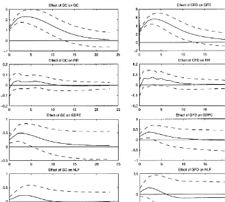
2.1. Total hours worked
To examine the e!ect of a government spending shock on total hours worked, we examine two alternative speci"cations ofZ,
Z"[GC RR GDPC N¸F]@,
Z"[GFD RR GDPC N¸F]@.
The impulse responses of the VAR models are plotted in Fig. 1. Solid lines represent the point estimates, while dashed lines denote plus and minus two standard deviation bands.5
The graphs of the impulse responses for the two measures of government spending show that a positive innovation in government spending increases output and total hours worked. The interest rate declines in the"rst period and then starts increasing. However, the changes of neither total hours worked nor interest rates are statistically signi"cant within two standard deviations. The responses to di!erent spending shocks are qualitatively similar. These responses are consistent with the theoretical results of Aiyagari et al. (1992).
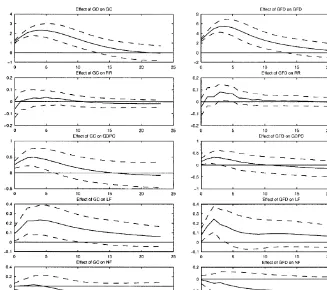
2.2. Employment and hours worked per worker
In this section, total hours worked are decomposed into the number of employees (NF) and the hours worked per worker (¸F). Two speci"cations of Zare considered,
Z"[GC RR GDPC ¸F NF]@,
Z"[GFD RR GDPC ¸F NF]@.
The impulse response functions of VAR models are plotted in Fig. 2. The responses of each variable to the shocks of di!erent measures of government spending are qualitatively similar. Employment and hours worked per worker respond di!erently to a shock in government spending. Hours worked per worker respond to the shock quickly and the changes are statistically signi"cant for the"rst several quarters under both measures of government expenditures. The time path increases for about 6 quarters and then declines. Employment responds slowly but the changes are more persistent. After an increase in government spending, employment decreases in the"rst two quarters, increases in the second half of the third quarter, and then decreases again, but the changes are not statistically signi"cant though the decreases after one year are almost
5These estimates are computed using the Monte Carlo method described in Doan (1992, example 10.1), using 500 draws from the estimated asymptotic distribution of the VAR coe$cients and the covariance matrix of the innovations,u
Fig. 1. VAR: the e!ect of government spending shocks on total hours worked.
signi"cant. The decrease in employment to an innovation in military spending is monotone and close to statistically signi"cant after two years.
These results are robust to two kinds of perturbations. One is changing the ordering of the variables inZ. The experiments show that the responses of each variable are very similar with di!erent positions of government spending in the ordering. Second, the results are qualitatively similar for a di!erent measure of hours worked, that is, data from a household survey. The responses using household survey data show a larger decrease in employment and a smaller increase in hours worked per worker than those from establishment data.
Fig. 2. VAR: the e!ect of government spending shocks on employment and hours worked per worker.
lowers employment in eight countries.6The paper also"nds that the multipliers of transitory changes in government spending are generally small: for a repre-sentative country, a one per cent transitory increase raises output by only 0.1 per cent.
The employment e!ect of military spending of the VAR model is consistent with the "ndings of some other empirical work. Dunne (1991) provides an analysis of military spending and unemployment for 14 OECD countries. The results suggest that fears that cuts in military spending will lead to an increase in unemployment are unjusti"ed, and he shows that disarmament presents an economic opportunity rather than a problem. Abell (1990) brings US time series
evidence to bear on the relationship of defense spending and unemployment rates. The analysis indicates that the increase in defense spending during the 1970s was associated with the improvement in the overall unemployment rate. However, during the 1980s, such increases were associated with a worsening of the unemployment rate.
Summarizing the results of our VAR analysis, we "nd that: total hours worked responds positively to increases in government spending; However, if total hours worked is decomposed into employment and hours worked per worker, we see that a spending increase leads to di!erent responses in these two components. More speci"cally, hours worked per worker responds to the shock more quickly than employment and increases in the "rst several periods and then decreases. On the other hand, employment stays at the same level in the
"rst several periods and then gradually decreases. Finally, the changes in employment are more persistent than hours worked per worker.
3. A stochastic general equilibrium model with a matching mechanism
The model economy includes households,"rms and government. The house-hold's employment status is determined by a lottery mechanism. It is assumed that there is an insurance market in the economy such that agents can insure themselves fully against idiosyncratic risks. This assumption makes households ex-ante identical and simpli"es the analysis. Firms create vacancies in the labor market and some vacancies are"lled through a matching mechanism. In each period, some existing jobs are destroyed exogenously. The di!erence between the"lled vacancies and the job separations is the increment in employment.
3.1. Households
The economy has a large number of in"nitely lived households. The popula-tion size is normalized to 1. Each household has capital gooda
twhich can be rented to a"rm and a unit of time which can be divided into working hours h
tand leisure 1!ht. The household derives utility from consumption goods,ct, and leisure, 1!h
t. The momentary utility function at timetis given by
;(c
t)#mH(1!ht),
wheremis a constant parameter and ; andH are assumed to be increasing,
concave and twice continuously di!erentiable.
A household's employment status is determined in each period via a lottery mechanism similar to the one described by Hansen (1985) and Rogerson (1988). Assume there exists a competitive and costless insurance market. At the begin-ning of each period, households may purchaseb
p
tper unit, wherebtis the quantity of the consumption good which is delivered to the household contingent on unemployment during that period.
In periodt, there aren
tavailable jobs to be rationed among the population. For each individual, the probability of being employed equalsn
t. Households lend their capital stock atu
t, and provide their labor,ht, if they are employed. The budget constraints of agents are contingent on their employment status. In the following constraints, subscript 1 represents the status of being employed, and 2 represents the status of being unemployed. Denoted
kas the depreciation rate of capital stock,w
tas the wage rate,utas the rental rate of capital stock, and a
tas the quantity of the capital asset. If the agent is employed, his income is composed of wage income (w
tht), rent (uta1,t), dividend payment (nt) and transfer payment from government (¹
t); the income is allocated among consumption (c
1,t), investment (a1,t`1!(1!dk)a1,t), and payment of insurance premium (p
tbt). Thus the budget constraint for an employed agent is c
1,t#a1,t`1!(1!dk)a1,t#ptbt4wtht#uta1,t#nt#¹t.
Similarly, an unemployed agent's income is composed of receipt of insurance payment, interest, dividend payment and net transfer from government; and the income is allocated among consumption, investment and insurance premium. The budget constraint for an unemployed agent is
c
2,t#a2,t`1!(1!dk)a2,t#ptbt4bt#uta2,t#nt#¹t.
The household's problem is to maximize the expected discounted utility,
E
tthat the household is employed, and with probability (1!nt) that the household is unemployed, subject to the above employment contingent budget constraints, where the agent takesMw
t,ut,nt,ntNas given.
In the presence of a costless competitive insurance market, it can be shown that households choose to insure themselves fully in equilibrium. Consequently, the agents are ex ante identical, and c
1,t"c2,t, a1,t"a2,t, bt"wtht, pt" (1!n
t).
Given that the agents are ex ante identical, the household's optimization problem can be rewritten as where the household takesMn
Two kinds of disturbances will be introduced later: a technology shock and a government spending shock. The government spending shock is of particular interest in this paper.
The Lagrangian associated with the household's optimization problem is
¸
0 is given and jt is the multiplier attached to the t-period resource constraint.
The e$ciency conditions are
;@(c fort"0, 1,2,Rand the transversality condition is
lim jt represents the shadow value ofc
t. The equation states that the household equates the marginal utility of datet's consumption to its opportunity cost in terms of utils. Eq. (1b) equates the marginal utility of leisure to the value of foregone earnings. The opportunity cost of investment is equal to its future discounted returns in (1c). Eq. (1d) is the budget constraint.
3.2. Firms
In each period, a "rm's economic activities include renting capital service, hiring workers, creating job vacancies, organizing production and selling products.
A"rm employs many workers, and on average, it is large enough to eliminate all uncertainty about the #ow of its labor force. The "rm's labor force is determined by the in#ow, new hires, and the out#ow, separations. The separ-ation rate,dn, is exogenous and constant over time.
The "rm creates vacancies (o
speci"cally,
m
t"htot.
The success rate is exogenous to the"rm, and it is governed by the e$ciency of the matching process in the labor market. For the "rm, the law of motion of employment (n the#ow from employment to unemployment.
Creating a vacancy is costly and the"rm has to spend resources on each job opening. The recruiting cost embodies the cost incurred when the"rm advertises the job opening, recruits candidates, trains the successful candidate and organ-izes his job. In the dynamic equilibrium, vacancies re#ect recruiting e!ort and change in response to expectations about pro"tability.
The "rm's output q
t is determined by a Cobb}Douglas production technology:
q
t"f(kt,ntht;zt)"kat(ztntht)1~a, where
k
t"capital stock at periodt, h
t"hours provided by a worker, z
t"an aggregate exogenous shock to technology, and 0(a(1.
We assume thez
tprocess is a logarithmic random walk with drift: ln(z
t)"ln(zt~1)#ln(z)#ez,t,
where the innovation, ez,t, is assumed to be identically and independently distributed through time with zero mean. The growth rate of this economy is ln(z).
A"rm's pro"t is the di!erence between the revenue from the sale of output and the cost of hiring labor, renting capital services and creating vacancies. We treat output as the numeraire, all factor prices are relative prices. The"rm's pure pro"t in periodtis
nt"q
t!utkt!wtntht!itot, where
u
t"rental rate of capital service att, w
t"wage rate at t,
Given the pricesM(u
t,wt,it)N=t/0, the separation ratedn, the success ratehtand the initial labor forcen
0, the problem faced by a"rm is to choose the amount of
capital services, the number of vacancies and outputM(k
t,ot,qt)N=t/0that
maxi-mize the present value of pro"ts. Thus its decision problem is
maxE
The Lagrangian of the"rm's problem is
¸ The e$ciency conditions are the following:
f The act of job creation is a decision by the"rm to"ll a vacant job at some cost. In equilibrium, the aggregate number of vacancies adjusts to eliminate any rent attributable to holding a job vacancy. Eq. (2b) is a free-entry condition. It equates the recruiting cost of a vacancy to the expected present value of holding a vacancy. The variablegtcan be explained as the capital value of a hired worker to the"rm.7Eq. (2c) de"nes the shadow valuegtas the pro"t the new worker will make to the "rm at t#1 plus the expected shadow value which is 0 with probabilitydnif the worker separates from the"rm, and isgt`1if he remains to work in the following period.
7This becomes clear if we write out the complete expression from (2c)
g
In each period, the"rm realizes some economic rent,f
2h!wh, from a retained worker. The worker hired attwill remain in this"rm att#1 and has probabilityd
nto leave the"rm in the periods after.
Thusg
The Euler conditions satis"ed by the optimal sequences ofk
We observe that if it"0, Eq. (3b) would reduce to the standard marginal productivity condition for employment.
3.3. Job matching and wage determination
According to Blanchard and Diamond (1989), the labor market in the US is highly e!ective in allocating workers to jobs. The#ows are large in proportion to stocks. The average duration of unemployment rarely exceeds 3 months; and the average duration of vacancies does not exceed a month. This implies the simultaneous coexistence of unemployment and vacancies. The study of worker
#ows to and from employment has generated a considerable literature.8The theoretical foundation of the matching process arises out of search and match-ing theory (see Pissarides, 1990). The basic idea is that the recruitmatch-ing e!ort of employers and the search e!ort of workers serve as inputs in a market matching function that generates new hires. The job vacancies and unemployed workers that are matched at any point in time are randomly selected from the setso
tand 1!n
t. (1!nt)/otis a measure of labor market tightness.
In this paper, we assume that all the unemployed workers search for jobs.9
The rate at which vacant jobs and searching workers match is determined by an increasing, concave, and homogeneous of degree one functionm(o
t, 1!nt) where o
t and 1!nt, respectively, represent the number of jobs that employers are attempting to "ll, and the number of workers seeking those jobs. Under the assumptions of random matching and constant returns, the probabilistic rate at which vacancies are"lled isht"m(o
t, 1!nt)/ot"m(1, (1!nt)/ot). The process that changes the state of a vacant job is Poisson with rateht. The mean duration of a vacant job is 1/ht. Unemployed workers move into employment according to a Poisson process with rate m(o
t, 1!nt)/(1!nt)"htot/(1!nt). The mean duration of unemployment isd
t"(1!nt)/mt.
8Devine and Kiefer (1991) include an extensive review of panel-based studies. Mortensen and Pissarides (1993) and Mortensen (1994) study the interaction of job creation and job destruction in a dynamic stochastic equilibrium framework.
In this paper, we assume the matching process is governed by a well behaved Cobb}Douglas matching function,10
m(o
t, 1!nt)"sott(1!nt)(1~t)4minMot, 1!ntN.
The wage rate is determined by decentralized bargaining between workers and"rms. The match between the worker and the "rm creates a surplus that must be bargained over. The wage rate is given by implicit bargaining at the individual level. The outcome of the bargaining is simply assumed as
w
t"(1!c)f2(kt,ntht;zt),
wherecis a constant (0(c(1) and a measure of the bargaining power of the
"rm. Thus, the wage rate is proportional to hourly productivity. The standard model equates the wage rate to the marginal product of labor. Thus the wage equation in the standard model can be viewed as a special case of the wage equation in this paper (c"0).
Firms spend resources on hiring, and this activity is an economic one just like production. To be consistent with balanced growth, recruiting cost per vacancy
it is assumed to have the same growth rate as the technological level z t. In a detrended economy, the recruiting cost is constant,it"i.
Eq. (2b) is then rewritten as
! itot
Government spending is exogenous. The government"nances its consump-tion solely by lump-sum taxaconsump-tion. This paper does not consider distorconsump-tionary
10The matching function in this paper is assumed to be constant returns to scale. According to Blanchard and Diamond (1989), there is empirical evidence suggesting constant or mildly increasing return to scale. The assumption of inequality in our matching function implies that the mean duration of vacancyo
t/htis more than one month and also the mean duration of unemployment
(1!n
t)/htis more than one month. There is no question about the assumption that the mean
taxes. The government faces the following budget constraint
g
t#¹t"0.
3.5. A competitive equilibrium
Dexnition.A competitive equilibrium is a set of pricesMu
t,wtN=t/0, an allocation
M(c
t,at,ht,nt)N=t/0 for a typical household and an allocation M(kt,ot,nt)N=t/0 for
a representative"rm, given exogenous sequences of technology shocks,Mz tN=t/0
t satis"es the bargaining solution;
4. government's budget constraints are satis"ed; 5. all markets clear,
a
t"kt, ht"m(ot, 1!nt)/ot.
The equilibrium conditions are summarized as follows:
;@(c These equations are used in GMM to get the estimates of the parameters.
4. Estimation method(GMM)and data measures
The Generalized Method of Moments (GMM), developed by Hansen (1982) and Hansen and Singleton (1982), is used to estimate the model. Like Christiano and Eichenbaum (1992), Burnside et al. (1993) and Burnside and Eichenbaum (1996), we use an exact identi"ed GMM estimator.
The GMM criterion is set up so that the estimated model exactly matches the sample analog of certain unconditional moments of the data generating process.
Government spendingg
tis assumed to be exogenous, following the process ln(g
whereg8t is the trendless component ofg
t. g8t has zero mean and follows ln(g8
t)"ogln(g8t~1)#egt,
where DogD(1,egt is the innovation in ln(g8t) with zero mean and standard deviationpg. This speci"cation implies that government spending grows at the same rate as that of total output so that a balanced growth path exists.
The structure parameters in the models are: Preference:b, m to 2 such that the share of recruiting cost is around 4%. Alternatively,ican be estimated by setting the value ofc, which re#ects the bargaining power of a"rm. Larger c indicates greater bargaining power for a "rm. c and i are closely related. A highercmeans more pro"t to the"rm, so the"rm can spend more in recruitment, thus allowing a larger i. t is set to 0.6, a value estimated by Blanchard and Diamond (1989) based on the 1968}1981 sample period.
4.1. The moment restrictions underlying the GMM estimator
The time series used in GMM include private consumption,c
t, gross invest-ment,i
t, capital stock,kt, government spending,gt, employment rate, nt, hours per worker, h
t, vacancy rate, ot, and average duration of unemployment, dt. (Appendix A contains a detailed explanation of these series.)
Di!erent from previous studies, output in this model equals aggregate de-mand plus resource costs in labor market search, i.e. the summation ofc
t,it, gt andi
tot. qtis not directly observable because data on recruiting costs are not available. We adopt the following strategy to solve this problem. As assumed earlier, recruiting cost per vacancy has to grow at the same rate as the techno-logy levelz
tto meet the requirement of balanced growth. In this model,qtalso grows at the same rate. So we assumeit is proportional to q
t, it"iqt. Then output can be written in terms of available time series and a parameteri, i.e. q
t"The parameter(ct#it#gt)/(1d!iot).
kis identi"ed by a condition E[ln(d
kt)!ln(dk)]"0, (5) wheredkt"1#(i
t!kt`1)/kt.
The parameterais identi"ed by the intertemporal Euler equation
E[1/b!(aq
By assuming thez
tprocess as follows: ln(z
t`1)"ln(zt)#ln(z)#ez,t`1,
and the production function, the technology shock is derived as
ln(z t)"
1
1!a[ln(qt)!aln(kt)]!ln(ntht).
ln(z) can be identi"ed by the balanced growth restriction which says that the mean growth rate of output coincides with that of technology.
E[ln(q
t)!ln(qt~1)!ln(z)]"0, (7)
alsopzcan be identi"ed from the condition,
E[(ln(z
t)!ln(z)!ln(zt~1))2!p2z]"0. (8) The parametermis identi"ed through the intratemporal e$ciency condition,
E
C
m!(1!c) (1!a)1!htNow we are going to identify i. From the Cobb}Douglas production function, we have
f
2(kt,ntht;zt)"(1!a)qt/(ntht), R
t"1!dk#aqt/kt.
Rewrite the Euler equation (3b) ofn tas EM!io
t/nt`1!(1!dn)nt(1!dk#aqt`1/kt`1)#qt`1/qt((1!a)c/nt`1
#(1!d
n)iot`1/nt`2!(1!dn)nt`1)N"0. (10)
Now consider government spending. The stationary component ofg
t,g8t, can
Finally the following two moment conditions are used to estimatednands, estimated by GMM. We have 11 parameters in W to be estimated and 11 moments conditions, Eqs. (5)}(15), thus forming an exact identi"cation system. The application of GMM requires that each equation includes only stationary variables. The moment conditions relating toWalready satisfy the requirement, becausec
t,qt, kt and gt all grow at rate ln(z), andnt, ht and ot are stationary. Therefore the variables involved dkt, q
t/kt, ct/ct`1, qt/ct, (1!ht)/(ntht), o
t/nt, qt`1/qt, andnt~1/ntare stationary.
4.2. Data measures
The following time series are expressed in quarterly real per capita terms. Detailed data description is given in Appendix A.
Private consumption,c
t, is measured as personal expenditure on nondurable goods plus services. Government spending,g
t, is measured by real government purchases of goods and services. The capital stock, k
t, is measured as a net, end-of-period stock consisting of non-residential, "xed capital owned by the private and government sectors plus government and private residential capital, and consumer durable goods. Gross investment,i
t, is measured as the sum of private investment and government investment corresponding to the above capital stock. The employment rate,n
t, is measured as the ratio of the number of employed persons to the non-institutional population, aged 16 and over. Aver-age working hours,h
t, is measured as the ratio of the aggregate hours of wage-and salary-earning workers in non-agricultural establishments to the number of persons employed. The vacancy rate,o
t, is measured as the ratio of help-wanted advertising to the non-institutional population.
4.3. GMM estimation results
For the purpose of comparison, a version of the Burnside et al. (1993) labor hoarding model is also considered and referred as thebenchmark model.11In the original BER model, e!ort is#exible and the shift length is"xed. To facilitate comparison, we reinterpret e!ort to be hours worked per worker and set shift length to be one. Appendix B presents a more detailed description of the BER
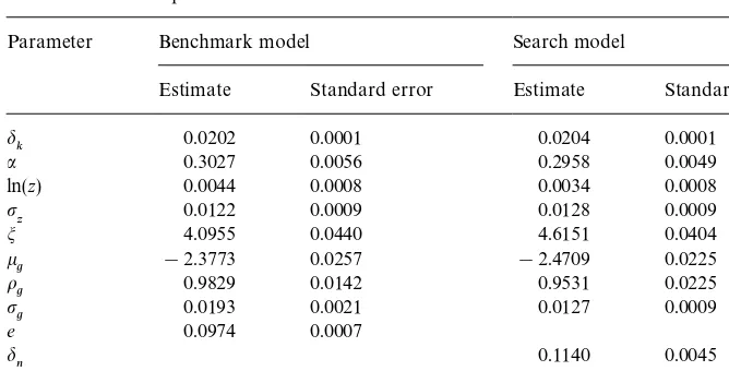
Table 1
GMM estimates of parameters in the benchmark and search models Parameter Benchmark model Search model
Estimate Standard error Estimate Standard error
d
k 0.0202 0.0001 0.0204 0.0001
a 0.3027 0.0056 0.2958 0.0049
ln(z) 0.0044 0.0008 0.0034 0.0008
p
z 0.0122 0.0009 0.0128 0.0009
m 4.0955 0.0440 4.6151 0.0404
k
g !2.3773 0.0257 !2.4709 0.0225
o
g 0.9829 0.0142 0.9531 0.0225
p
g 0.0193 0.0021 0.0127 0.0009
e 0.0974 0.0007
d
n 0.1140 0.0045
c 0.0657 0.0022
s 0.9602 0.0404
model. The parameters in the BER model to be estimated include
Md
k,a,m, ln(z),pz,kg,og,pg,eN, whereeis a "xed cost to go to work in terms of hours of foregone leisure. The model developed in Section 3 above is referred as thesearch model. The parameters of the benchmark model and the search model are estimated using the same data set. Model parameter estimates and standard errors are reported in Table 1.
The estimate of the capital depreciation rate for both models is 0.02. The capital share of output,a, is estimated to be around 0.30. These estimates are similar to those in Christiano and Eichenbaum (1992) and Burnside and Eichen-baum (1996). The separation rate,dn, is estimated to be 0.11. In steady state, the average duration of a job advertisement is equal to o/dnn"0.29 month. The matching e$ciency coe$cient in the matching function,s, is estimated to be 0.96.
5. Near steady state dynamics of the model
In order to examine the dynamic responses of the economy to di!erent persistence levels of government spending shocks, we adopt the method of King, Plosser and Rebelo (1990) to determine the near steady state dynamics of the model.
In this model, there are two state variables, the capital stockk
tand employ-mentn
the"rm's problem. For control variables, the households decide on consump-tionc
tand hours worked per workerht, and the"rm decides on vacanciesot. By the law of motion of the labor force, vacancies can be expressed in terms of employment, thus the problem can be rewritten to have four state and co-state variables and two control variables.
In the following analysis based on the search model, four kinds of shocks with di!erent degrees of persistence are considered: a transitory shock (o
g"0); persistent shocks, (o
g"0.93), (og"0.95) and (og"0.97), where (og"0.95) cor-responds to the GMM estimate in the last section, and (o
g"0.93) and (o
g"0.97) correspond to minus-one and plus-one standard deviations in the persistence level. Also, we will compare the VAR model to the search model which has (og"0.95).
In the benchmark model, we also consider four kinds of shocks with di!erent degrees of persistence: a transitory shock (og"0); persistent shocks, (og"0.98), (og"0.97) and (og"0.99), where (og"0.98) corresponds to the GMM estimate in the last section, and (og"0.97) and (og"0.99) are close to minus-one and plus-one standard deviations.
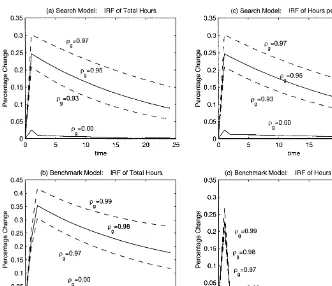
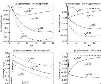
Figs. 3}6 plot the dynamic responses of selected variables in the bench-mark and search models to a one-standard-deviation shock to government consumption.
5.1. Total hours worked
In the benchmark model with a positive income e!ect on leisure, persistent changes in government spending always have an e!ect on total hours worked and output that is larger than the e!ect of transitory changes. The response functions in Fig. 3(b) show that a transitory shock (og"0) increases hours by 0.02%, while persistent shocks (og"0.98) increase hours by 0.35%.12 The reason is well explained in Aiyagari et al. (1992). Holding private investment constant, the e!ect of government spending on hours worked is positive due to a negative wealth e!ect. A transient increase in government spending reduces investment, but a persistent increase in government spending either increases investment or does not reduce it by as much as in the transient case. Thus persistent changes in government spending generate larger contemporaneous e!ects on both hours worked and output than transient changes.
Fig. 3. Impulse response functions of total hours and hours worked per worker.
Fig. 3(a) plots the impulse responses of total hours worked in the search model. These responses are the combination of the responses of employment and hours worked per worker which we will explain in the next section. The time paths of total hours worked are similar to those in the benchmark model, but with smaller magnitudes.
5.2. Employment and hours worked per worker
Fig. 4. Impulse response functions of employment.
steady-state level since, in the steady state, increasing employment reduces an agent's expected utility less than increasing the hours worked per worker. (Utility is linear over employment, but convex over e!ort.)
In the search model, hours worked per worker and employment respond di!erently to a government spending shock (Figs. 3(c) and 4(a)). The shock a!ects them through di!erent mechanisms. Hours worked per worker are determined by the household through intertemporal substitution. Employment is determined by job destruction and creation in the labor market. Changes in employment in this model depend crucially on the decision by the"rm to create a vacant job at some cost. In the dynamic equilibrium, vacancies re#ect recruit-ing e!ort and move in response to the expectation of the pro"tability of a successful match.
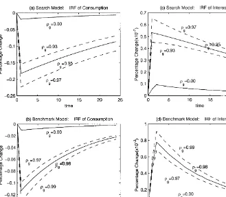
Fig. 5. Impulse response functions of consumption and interest rates.
Compared to the response of hours worked per worker, employment re-sponds to the shock slowly. The transitory shock (og"0) decreases employ-ment, and employment reaches its lowest point six periods after the shock, then employment increases gradually and eventually returns to its steady state value.13
The explanation of employment behavior is as follows. In this model, job creation is determined by job openings of the "rm. The "rm increases or decreases job openings based on the expected capital value of a hired worker to the"rm. A higher value of a hired worker to the "rm encourages the"rm to create more vacancies. The capital value of a hired worker to the "rm is the expected discounted economic rent that a worker brings to the"rm. There are
13A persistent shock may decrease or increase employment depending on the degree of the persistence. Numerical experiments show that a random walk government spending shock with (o
Fig. 6. Impulse response functions of wage rates and GDP.
two factors that a!ect the capital value. One is real interest rate and the other is the pure economic rent in each period. Higher interest rates lower the expected capital value of a hired worker. Higher economic rent increases the capital value. Negative wealth e!ects bring private consumption below its steady state value in the impact period, and then consumption gradually returns to its steady state value (Fig. 5(a)). The convergence is monotonic.14 Under the demand shock, there exists excess demand in the goods market at the prevailing interest rate, and the interest rate must go up to clear the goods market (Fig. 5(c)). The model shows that an increasing private consumption time path from below the steady state is accompanied by an above steady state average interest rate.
A worker's economic rent is determined by his/her productivity and hours. A shock may either increase or decrease economic rent, because the response of
14A shock may crowd in or crowd out private investment depending on the value of o
g.
Numerical experiments show that a temporary shock with persistenceo
gclose enough to one crowds
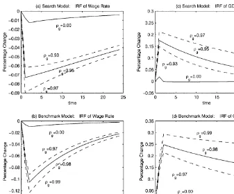
the productivity of labor may be opposite to that of hours (Fig. 6(a) and (b)). The
"gures show that even though economic rent increases to a shock with 0(o
g40.97 (Figs. 3(a) and 6(a)), the negative interest rate e!ect on the capital value still dominates the positive economic rent e!ect. Thus the expected capital value decreases and vacancies are less (Fig. 4(c) and (d)).15 In Fig. 4(a), the employment levels for shocks with higher persistence levels (og"0.93, 0.95) are lower than that for a transitory shock (o
g"0). We also observe that the employment levels with (o
g"0.95, 0.97) are above that of (og"0.93).
We can understand the above observation by viewing the responses of the shadow values of a hired worker and vacancies (Fig. 4(c) and (d)). The shadow value corresponding to a shock with (og"0) is higher than those of (o
g"0.95) and (og"0.97); and the shadow values for (og"0.95) and (og"0.97) are higher than the one with (og"0.93). Correspondingly, the case with the transitory shock has more vacancies than the cases with (og"0.93) and (og"0.95), and the cases with (og"0.95) and (og"0.97) have more vacancies than the case with (og"0.93).
5.3. Output ewects
The output e!ects are similar in these two models (Fig. 6(c) and (d)). A shock in government spending always increases output, with more persistent shocks leading to greater increases. That is, we observe multiplier e!ects with persistent government spending shocks. In the search model, an increase in government spending unambiguously raises hours worked per worker, but may increase or decrease the capital stock and employment. The results indicate that the positive hours e!ect dominates the other two e!ects regardless of the persistence of the shock.
5.4. Comparison of hours and employment ewects of the search model and VAR models
Another comparison is between the VAR models in Section 2 and the search model with a shock (og"0.95) using the GMM estimate. In the search model, a one standard deviation increase in government spending increases hours worked per worker by 0.25% in the impact period, and then hours worked per worker gradually returns to the steady state. In the VAR models, hours worked per worker increase by 0.24% during the"rst 5 quarters and then decrease.
The employment time paths of these two models are similar, employment gradually decreases in the two models after a shock, and reaches its lowest level in the 15th to 20th quarters. But the decrease in the search model is much smaller in magnitude than that in the VAR models. However, the employment
15However, for shock witho
gclose enough to 1, the positive rent e!ect dominates the negative
response in the VAR models is not signi"cantly di!erent from zero. Thus, qualitatively, the search model can generate similar responses of employment and hours worked per worker to those in the empirical VAR studies.
6. Conclusions
This paper focuses on the e!ects of temporary government spending shocks in the US economy on employment, hours worked per worker and output. Several VAR models demonstrate that a temporary innovation in government spending raises both hours worked per worker and output, but lowers the employment level. We construct a stochastic general equilibrium model in which employ-ment is determined by a matching mechanism. The results show that, in contrast to a reinterpreted Burnside, Eichenbaum and Rebelo's (1993) labor hoarding model, the search model can generate similar responses of hours worked per worker and employment to those of VAR models.
Acknowledgements
We would like to thank Andreas Hornstein, Jonas Fisher, Joel Fried, John Knight, Audra Bowlus, Ben Fung, Walter Engert, Peter Howitt, Dan Peled, Pierre Sarte, two anonymous referees and participants at seminars at the University of Western Ontario and the University of Calgary for helpful com-ments and suggestions. The Ontario Government is acknowledged for its
"nancial support by the "rst author. This paper represents the views of the authors and should not be interpreted as re#ecting those of the Bank of Canada, the Federal Reserve Bank of Richmond or the Federal Reserve system. Any errors are our own.
Appendix A. Data source description and transformation
A.1. Raw data source and series
(1) U.S. National Income and Product Accounts Tables, Bureau of Economic Analysis, U.S. Department of Commerce. Quarterly data. In 1987 dollars (Billions).
CC}Personal Consumption Expenditures
GC}Government Purchases of Goods and Services
GFD}Federal National Defence (de#ated by GDP de#ator) GDPC}Gross Domestic Product
(2) Fixed Reproducible Tangible Wealth in the U.S. tables. Bureau of Eco-nomic Analysis, U.S. Department of Commerce. Annual data. In 1987 dollars (Millions).
NBNTIC}Nonres Pvt Cap, by Leg Org, Tot All Ind: Net Stock, Eq & Str IBNTIC}Nonres Pvt Cap, by Leg Org, Tot All Ind: Invest., Eq & Str NBNGOAMC } Nonres Gvt-Own, Pvt Oper Cap, All Agen-Mfg: Net Stk, Eq & Str
IBNGOAMC } Nonres Gvt-Own, Pvt Oper Cap, All Agen-Mfg: Invest., Eq & Str
NEDGTC}Consumer-Total Durable Goods: Net Stock, Eq IEDGTC}Consumer-Total Durable Goods: Investment, Eq
NBRTOTGC}Res Cap, by Legal Org, All Own, inc Gvt: Net Stock, Eq & Str IBRTOTGC}Res Cap, by Legal Org, All Own, inc Gvt: Invest., Eq & Str NBNGFC}Nonres Gvt-Owned Capital, Federal: Net Stock, Eq & Str IBNGFC}Nonres Gvt-Owned Capital, Federal: Invest., Eq & Str NBNSLC}Nonres Total State & Local Govt, Net Stock, Eq & Str
IBNGLC } Nonres Govt Capital: State & Local, Investment, Eq & Str
(3) Bureau of Labor Statistics, U.S. Department of Labor, seasonal adjusted monthly data.
LE}Civilians Employed (Thous)
LNAN}Employee Hours in Nonagricultural Est. (Bil. Hrs)
LHTNAGRA } Aggregate Hours of Wage and Salary Workers in Nonagr Estab (Bil. Hrs)
LENA}Civilians Employed: Nonagricultural Industries (SA, Thous.) LR}Civilian Unemployment Rate (%)
LP}Civilian Participation Rate (%)
LNN}Civilian Noninstitutional Population (NSA, Thous.)
RATADVHW } The Ratio of Help-wanted advertisings to Persons Unem-ployed (%)
(4) CANSIM
TBR}91-Day Treasury Bill yield (%)
A.2. Data transformation
The following series are in per capita terms:
i"(IBN¹IC#IBNGOAMC#IEDG¹C#IBR¹O¹GC
Appendix B. A version of Burnside et al.'s(1993)Labor Hoarding Model
The model economy is populated with a large number of in"nitely lived individuals. To go to work, an individual must incur a"xed cost,e, denominated in terms of hours of forgone leisure. Once at work, an individual chooses hours workedh
t. The time endowment is normalized to 1. The momentary utility at timetis given by
ln(c
t)#mntln(1!e!ht)#m(1!nt) ln(1) . (B.1) Output,y
t, is produced via the Cobb}Douglas production function y
t"kat(ztntht)1~a, (B.2) where 0(a(1,n
t denotes the total number of individuals going to work at timet, k
tdenotes the beginning-of-period capital stock,ztrepresents the growth rate of exogenous labor-augmenting technological progress and it evolves according to
lnz
t"lnzt~1#lnz#ezt, (B.3) whereeztis the innovation to lnz
twith a standard deviation ofpz. Firms commit to the number of workers employed before observing any shocks to the econ-omy. After observing the shocks, "rms can adjust the work hours of their employees.
The aggregate resource constraint is given by
c
t#kt`1!(1!dk)kt#gt4yt. (B.4) The parameter d represents the depreciation rate on capital. The random variableg
tdenotes timetgovernment consumption which evolves according to lng
t"lnzt#kg#lng8t, (B.5) whereg8t has the law of motion
lng8t"o
glng8t~1#egt, (B.6)
whereegtis the innovation to ln (g
The social planner chooses a set of stochastic processesMk
Except some notations, the only di!erence between this model and the one presented in BER is that instead of having agents choose e!ort with shift length
"xed, we treat the product of the two as the hours worked per worker which is a choice variable of the households.
References
Abell, J.D., 1990. Defence spending and unemployment rates: an empirical analysis of disaggregate by race. Cambridge Journal of Economics 14, 405}419.
Abraham, K., 1987. Help-wanted advertising, job vacancies and unemployment. Brookings Papers on Economic Activity 1, 207}243.
Aiyagari, S.R., Christiano, L.J., Eichenbaum, M., 1992. The output, employment, and interest rate e!ects of government consumption. Journal of Monetary Economics 30, 73}86.
Andolfatto, D., 1996. Business cycles and labor-market search. American Economic Review 86, 112}132.
Baxter, M., King, R.G., 1993. Fiscal policy in general equilibrium. American Economic Review 83, 315}334.
Blanchard, O., Diamond, P., 1989. The beveridge curve. Brookings Papers on Economic Activity 1, 1}76.
Burnside, C., Eichenbaum, M., 1996. Factor hoarding and propagation of business cycle shocks. American Economic Review 86, 1154}1174.
Burnside, C., Eichenbaum, M., Rebelo, S., 1993. Labor hoarding and the business cycle. Journal of Political Economy 101, 245}273.
Campbell, J.Y., 1994. Inspecting the mechanism. Journal of Monetary Economics 33, 463}506. Christiano, L.J., Eichenbaum, M., 1992. Current real-business-cycle theories and aggregate
labor-market#uctuations. American Economic Review 82, 430}450.
Devine, T.J., Kiefer, N.M., 1991. Empirical Labor Economics: The Search Approach. Oxford University Press, Oxford.
Doan, T., 1992. User's Manual, RATS Version 4. VAR Econometrics, Evanston, IL.
Dunne, J.P., 1991. Conversion and employment: a comparative assessment. DAE Working Paper 9116, University of Cambridge.
Hall, G., 1996. Overtime, e!ort, and the propagation of business cycle shocks. Journal of Monetary Economics 38, 139}160.
Hansen, G., 1985. Indivisible labor and the business cycle. Journal of Monetary Economics 16, 309}327.
Hansen, L.P., 1982. Large sample properties of generalized method of moments estimators. Econometrica 50, 1029}1054.
King, R.G., Plosser, C.I., Rebelo, S.T., 1990. Production, growth and business cycles: technical appendix. Mimeo, University of Rochester.
Merz, M., 1995. Search in the labor market and the real business cycle. Journal of Monetary Economics 36, 269}300.
Mortensen, D.T., 1994. The cyclical behavior of job and worker #ows. Journal of Economic Dynamics and Control 18, 1121}1142.
Mortensen, D.T., Pissarides, C.A., 1993. The cyclical behavior of job creation and job destruction. In: Ours, J.C., Pfann, G.A., Ridder, G. (Eds.), Labor Demand and Equilibrium Wage Formation. North-Holland, Amsterdam.
Pissarides, C.A., 1985. Short-run equilibrium dynamics of unemployment vacancies and real wages. American Economic Review 75, 676}690.
Pissarides, C.A., 1990. Equilibrium unemployment theory. Blackwell, Oxford.
van Ours, J., Ridder, G., 1992. Vacancies and the recruitment of new employers. Journal of Labor Economics 10, 138}155.