VA R I AT I O N I N T R E E C O M M U N I T Y C O M P O S I T I O N
A N D S T R U C T U R E W I T H C H A N G E S I N S O I L
P R O P E R T I E S W I T H I N A F R A G M E N T O F
S E M I D E C I D U O U S F O R E S T I N S O U T H - E A S T E R N
B R A Z I L
A. T. O -F *, N. C , E. A. V & D. A. C
The purpose of the present study was to investigate whether variations in tree community structure and soil properties were interrelated in a fragment of semideciduous forest in Martinho Campos, south-eastern Brazil. The forest was sampled by ten plots, each of which was made up of four contiguous 15×15m quadrats (total 0.9ha). Plots were randomly distributed in the fragment with the help of grid-line coordinates. Soil samples were collected from each quadrat for chemical and textural analyses, and the soil of each quadrat was classified in conformity with the US Soil Taxonomy System. All trees with diameter at the base of the stem5cm were identified and measured (circumference and height). Three soil groups were recognized: Ustifluvent, Ustropept, and Dystropept. A principal component analysis independently discriminated the soil groups in terms of their chemical and textural properties, indicating the consistency of the soil classification. Significant differences among the soil groups were also found for most soil properties. Tree community physiognomy was significantly different in Ustropept soil habitat, where trees showed more pronounced slenderness. A detrended correspondence analysis indicated that tree community structure also responded to the three soil habitats. A canonical
correspondence analysis, together with Spearman’s rank correlations, demonstrated that species’ abundance distributions were significantly correlated with the soil properties. Differences in soil nutrient content (particularly Ca2+and K+) and in ground water regime are apparently the leading factors determining tree species distributions within the fragment.
Keywords. Brazilian Atlantic forest, multivariate analysis, tropical semideciduous forest, tropical soils.
I
Spatial heterogeneity in the physical environment is an important factor causing the commonly high tree species diversity of tropical forests, as variations in resource availability in both horizontal (particularly soil chemical and textural properties and ground water regime) and vertical (canopy layering, rooting zones) aspects afford dimensions for niche differentiation among tree species (Fowler, 1988; Terborgh, 1992). The progress of the gap-phase dynamics theory for tropical forests (see
Denslow, 1987, for a review) has made clear that temporal heterogeneity of the environment plays an equally important role in determining tree species distribu-tions. In fact, the model of tropical forests as species mosaics with asynchronous pieces determined by diversity-promoting disturbance factors (e.g. Denslow, 1985; Oldeman, 1990) has dimmed, to a considerable extent, the notion that the substratum also plays an important role in determining the horizontal patterns of tree species distribution (Clarket al., 1998).
On a local scale, topography has been regarded as the most important substratum-related variable causing spatial variation in the structure of tropical forests because it commonly corresponds to changes in soil properties, particularly ground water regime and natural soil fertility (Bourgeron, 1983). The correlation between tree species distribution and topographic and soil variables has been successfully demon-strated in numerous studies of tropical forests world-wide (e.g. Gartlanet al., 1986; Newbery et al., 1986; Basnet, 1992; Johnston, 1992; ter Steege et al., 1993; Duivervoorden, 1996; Silva Ju´nior et al., 1996; Clarket al., 1998; Van den Berg & Oliveira-Filho, 1999).
The present contribution is one of a series of studies carried out of forest fragments in the state of Minas Gerais, south-eastern Brazil, with the main purpose of produc-ing information on the ecology of native tree species in order to assist environmental reclamation projects in selecting species for particular sites (Oliveira-Filho et al., 1994a,b,c, 1997a,b, 1998). These studies consist basically in determining preferential habitats of species in terms of both soil properties and light environment for establish-ment and growth (regeneration guild ). In this case we investigated the response of the tree community in a fragment of semideciduous forest to variation in particular soil properties in addition to other intervening factors, including stochastic effects. The sampling of the tree community and soil variables followed an inductive approach ( Kent & Coker, 1996), i.e. the sampling design was not influenced by an
a priorimodel of soil–vegetation relationships. This approach was successful in ident-ifying significant correlations among soil properties, soil classification categories, topography (drainage), and tree community structure.
M M
The study area
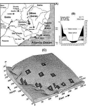
F I G . 1 . (A) Geographical situation of the municipality of Martinho Campos in south-eastern Brazil; (B) Walter climatic diagram for the region (data from DNMet, 1992), diagram follows Walter (1985); and (C ) surface grid showing the distribution of the ten sample plots (A to J ) on the study area. Lines on surface grid are spaced at 5m intervals; plots are made up of four adjacent 15×15m quadrats.
respectively (Fig. 1c). There was no evidence of serious human interference in the forest, and the owners informed us that they have been strict in protecting the area.
Forest and soil surveys
Sampling procedure followed the protocol of our previous studies (Oliveira-Filho
placed in the forest fragment with the help of a 5×5m grid with axes running N–S and E–W laid over the map of the area ( Fig. 1c). We located the SE corners of six plots from grid coordinates randomly taken within those situated at distances less than 15m from the northern margin of both the river and gully (valley bottom plots). Another six plots had their SE corners located at grid coordinates randomly taken within those situated at distances more than 40m from the river and gully (slope plots). We discarded two slope plots from the total sample because they coincided with large, recently formed canopy gaps and their floristic composition had a strong bias toward pioneer species. The ten remaining plots were divided into four 15×
15m adjacent quadrats. The relative location of quadrats was adjusted in some valley bottom plots to follow the contour of the river and rocky gully (see Fig. 1c).
We identified and measured the height and circumference at the base of the stem (cbs) of all trees occurring in the quadrats with a cbs 15.7cm (5cm diam.). For the few buttressed trees the cbs was recorded above the buttresses. Voucher specimens are lodged at the Herbarium of the Universidade Federal de Lavras ( ESAL).
We collected four 0.5L soil samples from a depth of 0–20cm at the midpoints between the corners and the centre of each quadrat. This depth greatly coincides with the highest concentration of roots in the local soil profile. The four soil samples were bulked and subsampled for each quadrat. Chemical and granulometric analyses were carried out at the Soil Laboratory of the Universidade Federal de Lavras (see laboratory procedures in Oliveira-Filho et al., 1994a,b). The soil of each quadrat was also classified in conformity with the US Soil Taxonomy System (Soil Survey Staff, 1996), resulting in three major soil groups. These were considered the distinct soil habitats of the tree communities.
Data analysis
We calculated mean values per plot for each soil variable (pH, P, K+, Ca2+, Mg2+, Al3+, total exchangeable bases, organic matter, and percentage sand, silt and clay) from the values obtained for the quadrats by the soil laboratory. Then we compared the soil variables in the ten plots among the three soil groups with ANOVAs, applying Tukey tests to those with significantFs (Zar, 1996). We used the means instead of the original values because quadrats within plots are actually pseudoreplications. A principal component analysis (PCA) of ten soil variables (all but total exchangeable bases) in the 40 quadrats was also performed to assess the consistency of the soil classification, and to identify the most strongly discriminating variables ( Kent & Coker, 1996). In this case we used the quadrat values instead of plot means to appraise within-plot variation.
individ-ual tree heights against log-transformed diameters and compared the slopes of the resulting curves with the Tukey–Kramer method (Sokal & Rohlf, 1981).
We used canonical correspondence analysis, CCA (ter Braak, 1987), to investigate the relationships between species abundance and environmental variables in the quadrats using the program CANOCO (ter Braak, 1988). The species-abundance matrix consisted of the number of individuals per quadrat. Only 33 species with10 individuals in the total sample were included in the matrix. As recommended by ter Braak (1995), all abundance values were log-transformed prior to matrix processing, as their distributions were skewed toward a few very large values. The matrix of environmental variables per quadrat initially included the same ten soil variables used in the PCA plus two additional variables. The distance from the quadrat centre to the nearest forest edge was included to assess edge-effects, as recent studies indicate that they may affect floristic patterns up to c.100m from edges (Laurance et al., 1998a,b). The vertical distance from the quadrat centre to the nearest valley bottom (either river or gully) was included to assess the influence of topographic sites on tree community. After a preliminary analysis, we eliminated five variables because of high redundancy (variance inflation factor >20) or poor correlation with ordi-nation axes (intraset correlations with the first two axes between−0.5 and 0.5, and t-values for canonical coefficients <2.1) (ter Braak, 1988, 1995). These were the vertical distance to the valley bottom (highly redundant with Ca and pH ), the distance to the forest edge and the levels of P, organic matter and silt. A Monte Carlo permutation test (ter Braak, 1988) was performed to assess the significance of the correlation between species abundance and the remaining seven soil variables. We performed a detrended correspondence analysis, DCA, with the species-quadrat matrix and indicated the soil habitats on the resulting species-quadrat ordination diagram to confirm the consistency of patterns emerging from the CCA (ter Braak, 1995). With a similar aim, we also calculated Pearson’s correlation coefficients, and their significance, between soil variables and log-transformed species abundance in the ten sample plots. Soil variables and species were the same used by CCA.
R
where the soil is very deep (>3m). Ustifluvents, Ustropepts and Dystropepts corre-spond to Eutric Fluvisols, Eutric Cambisols and Dystric Cambisols, respectively, in the FAO-UNESCO legend (Oliveira & Van den Berg, 1996).
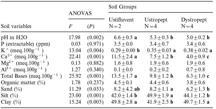
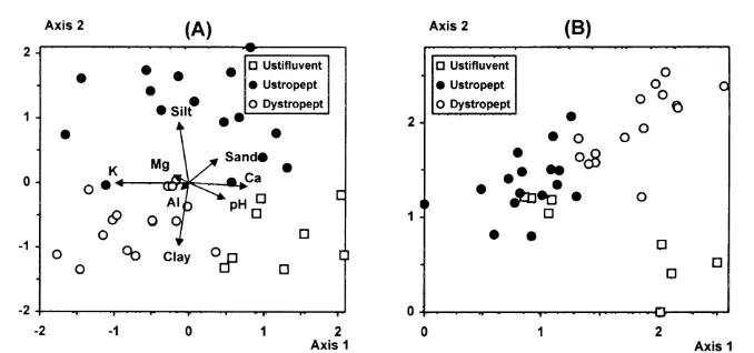
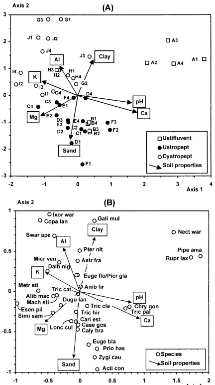
There were significant differences between the three soil groups for seven out of the 11 soil variables ( Table 1), indicating that the soil classification was highly con-sistent in terms of topsoil chemical and textural properties. Ustifluvents were the richest soils in Ca2+, reflected in the highest levels of total bases (eutric) shown. Soil pH was also the highest in Ustifluvents, but the levels of K+were the lowest. The amounts of Ca2+ (and related total bases) decreased towards Ustropepts (eutric) and Dystropepts (distric), while those of K+ increased. The proportions of sand were higher for Ustifluvents and Ustropepts, the latter also showing the highest and lowest proportions of silt and clay, respectively. The same trends appear in the PCA diagram where the quadrats of each soil group are clearly discriminated (Fig. 2a). The first component has a high eigenvalue (0.871) and accounts for most of the total variance of soil properties data (87.1%). It is highly correlated with Ca2+, pH (both positively), and K+(negatively), and discriminates most Ustifluvent quadrats from the other soil groups. Although the second component has an insignificant eigenvalue (0.091) and adds very little to the accumulated variance (96.2%), it clearly discriminates Ustropept quadrats and is more strongly correlated with the pro-portions of silt (positively) and clay (negatively).
Forest physiognomy was characterized by a canopy of irregular height (12–20m), dense understorey and intermediate deciduousness. During the dry season 15–25% of trees are totally leafless while the others only reduce the foliage. A total of 1512
TA B L E 1 . Soil variables in the ten plots of semideciduous forest classified into three soil groups. Figures are means±standard deviations. WhereFtests rejected the null hypothesis (P<0.05), means followed by different bold letters indicate significant differences in Tukey tests (P<0.05)
Soil Groups ANOVAS
Ustifluvent Ustropept Dystropept Soil variables F (P) N=2 N=4 N=4
F I G . 2 . Diagrams of quadrat ordination in the first two axes yielded by (A) principal compo-nent analysis of soil properties and (B) detrended correspondence analysis of species abun-dance. Quadrats are classified into soil habitats in both diagrams. Soil properties are given as arrows in the PCA diagram (arrows for P and organic matter are too small to be shown).
individual trees, 121 species and 41 families were registered. Ecological dominance was substantial: the ten species with the highest densities accounted for 52.7% of all individuals while the ten with the highest basal areas accounted for 51.5% of the total basal area (see Appendix).
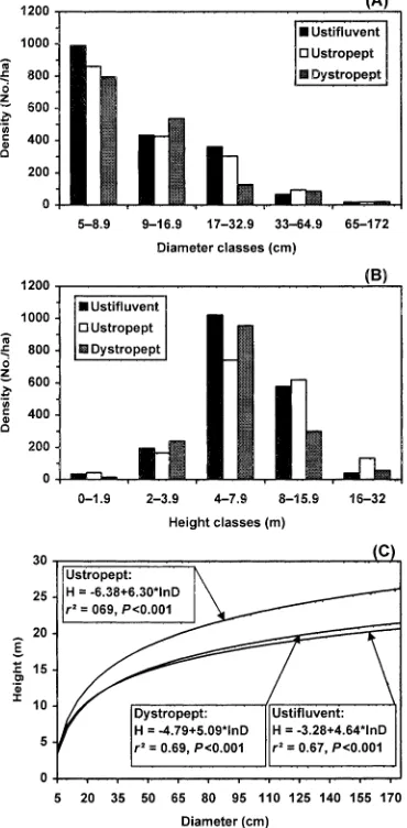
Size class distributions of trees (Fig. 3a,b) differed significantly among soil habitats for both diameters (x2=40.4,P<0.001) and heights (x2=78.9,P<0.001). The main contributions to the chi-square value for diameters were those from Ustropepts and their higher and lower frequencies in the 9–17 and 17–33cm classes, respectively, regarding the expected values. For heights, the main contributions were related to the 4–8m class, with lower and higher frequencies than expected for Ustropepts and Dystropepts, respectively, and the 8–16m class, with opposite trends. These diff er-ences suggest that Ustropepts have higher proportion of slender trees compared to the other soil habitats. Higher tree slenderness in this soil habitat is confirmed by the height–diameter relationships (Fig. 3c) which produced curves with significantly different slopes (F=27.9,P<0.001), with Ustropepts showing a significantly higher slope ( Tukey–Kramer test,P<0.05).
F I G . 3 . Tree heights and diameters in the three soil habitats, Ustifluvent, Ustropept and Dystropept: (A) distributions of tree densities per diameter class; (B) distributions of tree densities per height class; and (C ) curves obtained by regressing height (H ) on log-transformed diameter (d ).
data are normal in vegetation data and do not impair the significance of species– environment relations (ter Braak, 1988). In fact, CCA produced considerably high values for both species–environment correlations (axis 1=0.90, axis 2=0.79) and respective cumulative percentage variances (axis 1=34.1%, axis 2=57.8%). In addition, the Monte Carlo permutation test indicated that the species abundance and environmental variables were significantly correlated (F-ratio=3.73, P<0.01, first axis; F-ratio=2.02,P<0.01, overall test).
yielded by both DCA (Fig. 2b) and CCA (Fig. 4a). The only exceptions are quadrats B1–B4 ( Ustifluvent) which appeared among Ustropept quadrats suggesting a tran-sitional species composition. The emergence of similar patterns from the two methods is particularly meaningful, confirming that the species–environment relations indi-cated by CCA are naturally underlying the species data structure (DCA). The only important difference between the two methods is that the gradients summarized by the first two axes are reversed. This is certainly a result of the constraining of
cal axes, which adjusts the species variance to that of the linear combination of environmental variables.
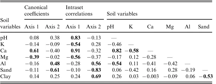
The first canonical axis was most strongly and positively correlated with Ca2+
and pH, followed to a much lesser extent by Mg2+ and K+, which were both negatively correlated ( Table 2 and Fig. 4a). As could be expected, Ca2+ was posi-tively correlated with pH and negaposi-tively correlated with K+. These trends correspond to the differentiation between Ustifluvent and the Inceptisols ( Ustropept and Dystropept) also identified by PCA ( Fig. 2a). The second canonical axis was more strongly influenced by the proportions of sand (negatively) and clay (positively), followed by Al3+. These trends coincide with the differentiation of Ustropept soils based on their coarser texture (see Fig. 2a and Table 1).
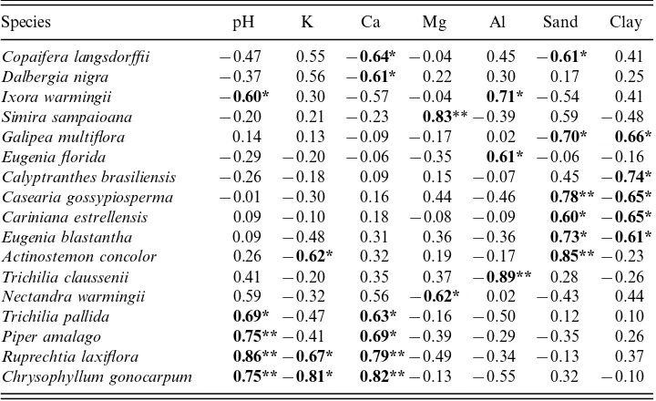
The species ordination by CCA (Fig. 4b) strongly agrees with their correlation coefficients with particular soil variables ( Table 3). Of the 33 species involved in the analysis, 17 showed significant correlation with at least one of the seven soil variables. Ca2+and sand produced the highest number of significant correlations (6), followed by pH and clay (both with 5), and clay (8). These were also the most strongly correlated variables with the first two canonical axes. The four species with positively significant correlations with Ca2+also appeared on the right side of the ordination diagram, and were also correlated with pH. The four species with positively signifi-cant correlations with sand are all concentrated on the bottom of the diagram. Three of these were also negatively correlated with clay.
D
Catenary variations of soil properties in tropical forests have commonly been attri-buted to topography itself, because variations in steepness and different topograph-ical levels on a slope may determine, to a great extent, different ground water regimes
TA B L E 2. Canonical correspondence analysis (CCA): canonical coefficients and intraset correlations in the first two ordination axes, and weighted correlation matrix for the seven soil variables supplied. Coefficients with t-values above 2.1 and correlations with absolute values>0.5 are enhanced in bold
Canonical Intraset
coefficients correlations Soil variables Soil
variables Axis 1 Axis 2 Axis 1 Axis 2 pH K Ca Mg Al Sand
TA B L E 3 . Pearson’s correlation coefficients (r) between the seven soil variables used in CCA and the log-transformed abundance of 17 species with at least one significantrvalue. N=10 plots with 900m2in area. Significantrvalues are given in bold
Species pH K Ca Mg Al Sand Clay
Copaifera langsdorffii −0.47 0.55 −0.64* −0.04 0.45 −0.61* 0.41 Dalbergia nigra −0.37 0.56 −0.61* 0.22 0.30 0.17 0.25 Ixora warmingii −0.60* 0.30 −0.57 −0.04 0.71* −0.54 0.41 Simira sampaioana −0.20 0.21 −0.23 0.83**−0.39 0.59 −0.48 Galipea multiflora 0.14 0.13 −0.09 −0.17 0.02 −0.70* 0.66* Eugenia florida −0.29 −0.20 −0.06 −0.35 0.61* −0.06 −0.16 Calyptranthes brasiliensis −0.26 −0.18 0.09 0.15 −0.07 0.45 −0.74* Casearia gossypiosperma −0.01 −0.30 0.16 0.44 −0.46 0.78**−0.65* Cariniana estrellensis 0.09 −0.10 0.18 −0.08 −0.09 0.60* −0.65* Eugenia blastantha 0.09 −0.48 0.31 0.36 −0.36 0.73* −0.61* Actinostemon concolor 0.26 −0.62* 0.32 0.19 −0.17 0.85**−0.23 Trichilia claussenii 0.41 −0.20 0.35 0.37 −0.89** 0.28 −0.26 Nectandra warmingii 0.59 −0.32 0.56 −0.62* 0.02 −0.43 0.44 Trichilia pallida 0.69* −0.47 0.63* −0.16 −0.50 0.12 0.10 Piper amalago 0.75**−0.41 0.69* −0.39 −0.29 −0.35 0.26 Ruprechtia laxiflora 0.86**−0.67* 0.79**−0.49 −0.34 −0.13 0.37 Chrysophyllum gonocarpum 0.75**−0.81* 0.82**−0.13 −0.55 0.32 −0.10
*P<0.05, **P<0.01.
and these, in turn, ordinarily affect soil texture and nutritional status (e.g. Richards, 1952; Bourgeron, 1983; Newbery & Proctor, 1984; Furley, 1992; Silva Ju´nioret al., 1996; Oliveira-Filho et al., 1997a; Van den Berg & Oliveira-Filho, 1999). In the present case, topography is strongly associated with the three soil habitats encoun-tered in the area and the corresponding variations in particular soil properties. Dystropepts are restricted to the mid and upper slopes, contrasting with Ustifluvents and Ustropepts, which are both situated on valley bottoms, although slopes are much steeper in the latter.
Total bases are highest in Ustifluvent, certainly because they are formed by rapid accretion of finer sediments and mineral nutrients depleted from other areas by drainage and flooding waters, while the intermediate levels found in Ustropepts probably results from the down-slope transport by drainage only (Crabtree, 1986; Hornung, 1990). However, this gradient results basically from a Ca2+ gradient, because this cation is the major responsible for the sum of bases. In fact, K+levels increased towards Dystropepts opposing the Ca2+gradient. This is probably a result of an increasing influence of the local bedrock in pedogenesis, because siltstones, slates, and other poor pellitic rocks in Brazil are normally poor in Ca and rich in K (Resendeet al., 1995). The coarser texture of Ustropepts is probably influenced by steep topography, which may cause proportionally higher losses of finer particles in the long run (McCaig, 1985).
in this study may lead to misinterpretations of the relative importance of certain soil factors. For instance, it is reasonable to think that the vegetation is responding to differences in ground water regime between the soil habitats as well as to their differences in nutritional status and soil texture. The strongly sloping topography of the Ustropept habitat, together with its coarser soil texture and shallow soil profile, certainly promote strong water shortage during the dry season. Therefore, if the Ustifluvent–Ustropept–Dystropept sequence represents a strong nutritional gradient, with increasing K+ and decreasing Ca2+ levels, the Dystropept–Ustifluvent– Ustropept sequence represents a no less important gradient of increasingly strong drainage and short water availability. Most studies carried out in the region with the same purpose and approach have suggested that floristic patterns were more strongly influenced by ground water regime than soil nutritional status (Oliveira-Filhoet al., 1994a,c,d, 1997a, 1998). This is the second case where soil fertility is apparently at least equally important (see Oliveira-Filhoet al., 1994b).
A number of species which were positively correlated with Ca2+, Mg2+, pH, or negatively correlated with Al3+, such as Trichilia pallida, Trichilia claussenii, Chrysophyllum gonocarpumand Simira sampaioana, have already been reported as showing preference for higher fertility soils in other areas (Ratter et al., 1988; Oliveira-Filhoet al., 1994b, 1998; Pinto, 1997). Among those negatively correlated with the same variables, Copaifera langsdorffii, Actinostemon concolor and Ixora warmingii have also been associated with low fertility soils (Oliveira-Filho et al., 1994b). Cariniana estrellensis and Casearia gossypiosperma, which were positively correlated with coarser soil texture ( Ustropepts), have also been associated with stronger soil drainage (Oliveira-Filhoet al., 1997a). This demonstrates that this type of study is capable of detecting patterns that, if repeatedly found in different areas, will produce solid information about the ecology of particular tree species.
The different soil habitats also produced variations in forest physiognomy within the forest fragment, with more pronounced tree slenderness in Ustropepts. Changes in tree size class distribution with soil drainage are commonly observed among tropical forests, but there seems to be no generalized pattern (Mantovaniet al., 1989; Oliveira-Filhoet al., 1990, 1994a,b, 1997a; Basnet, 1992). Although the present case could also suggest a relationship between tree slenderness and the stronger drainage of the Ustropept site, it is also possible that competition for light is the main factor behind the comparatively slimmer trees. As the Ustropept site resembles a gorge, the trees of the surrounding upper sites have an advantage in the competition for light and tend to cover those in the gorge, and these might respond by growing proportionally higher to compensate.
A
immensely grateful to our driver Roge´rio, and to the students Jose´ Roberto, Rubens Koloski, Gilce, Giuliana, and Warley, for their valuable help during field work.
R
B , K.(1992). Effect of topography on the pattern of trees in a tabonuco (Dacryoides excelsa) dominated forest of Puerto Rico.Biotropica24: 31–42. B , P. S.(1983). Spatial aspects of vegetation structure. In:G,
F.B.(ed.)Ecosystems of the World 14A – Tropical Rain Forest Ecosystems, Structure and Function, pp. 29–47. Amsterdam: Elsevier.
C , D. B. , C ,D. A.& R , J. M.(1998). Edaphic variation and the mesoscale distribution of tree species in a neotropical rain forest.J. Ecol.86: 101–112. C , R. W.(1986). Spatial distribution of solutional erosion. In: T, S. T.
(ed.)Solute Processes, pp. 239–361. Chichester: John Wiley & Sons.
D ,J. S.(1985). Disturbance-mediated coexistence of species. In:P,S.T.A. W,P.S. (eds)The Ecology of Natural Disturbance and Patch Dynamics,
pp. 307–323. New York: Academic Press.
D ,J. S.(1987). Tropical rainforest gaps and tree species diversity.Ann Rev. Ecol. Syst. 18: 431–451.
D N M (1992).Normais climatolo´gicas (1961–1990). Brası´lia: Ministe´rio da Agricultura, Departamento Nacional de Meteorologia (DNMet).
D ,J. F. (1996). Patterns of tree species richness in rain forest of the Middle Caqueta´ area, Colombia, MW Amazonia.Biotropica28: 142–158.
F , N.(1988). The effects of environmental heterogeneity in space and time on the regulation of populations and communities. In:D,A.J.,H,M.J.& W,A.R.(eds)Plant Population Ecology, pp. 249–269. Oxford: Blackwell Scientific Publications.
F , P. A.(1992).Notes on the Soils and Plant Communities of Fazenda A´ gua Limpa (Brası´lia, D.F., Brazil). Occasional Publications no. 5, Department of Geography, University of Edinburgh.
G ,J. S. ,N , D. M. ,T , D. W. & W ,P. G.(1986). The influence of topography and soil phosphorus on the vegetation of Korup Reserve, Cameroun.Vegetatio65: 131–148.
H , M. (1990). Measurement of nutrient losses resulting from soil erosion. In: H,A.F.,I,P.&H,O.W.(eds)Nutrient Cycling in Terrestrial Ecosystems, pp. 80–102. London: Elsevier Apl. Sc.
J , M. H. (1992). Soil–vegetation relationships in a tabonuco forest community in the Luquillo Mountains of Puerto Rico.J. Trop. Ecol. 8: 253–263.
K , M.& C , P.(1996).Vegetation Description and Analysis, a Practical Approach. London: Belhaven Press.
L , W. F. , F ,L. V. , R -D M , J. M. & L ,
S. G.(1998a). Rain forest fragmentation and the dynamics of Amazonian tree communities.Ecology79: 2032–2040.
L , W. F. , F ,L. V. , R -D M , J. M.e t a l. (1998b). Effects of forest fragmentation on recruitment patterns in Amazonian tree communities. Conserv. Biol. 12: 460–464.
MC , M. (1985). Soil properties and subsurface hydrology. In:R,K.S.,
A,R.R.&E,S.(eds)Geomorphology and Soils, pp. 121–140. London: George Allen & Unwin.
fitossociolo´gico de a´reas de mata ciliar em Mogi Guac¸u, SP, Brasil. In:B,L.M.
(ed.)Simpo´sio sobre mata ciliar, Anais, pp. 235–267. Campinas: Fundac¸a˜o Cargill. N , D. MC. & P , J. (1984). Ecological studies in four contrasting
lowland rain forests in Gunugu Mulu National Park, Sarawak. IV. Association between tree distribution and soil factors.J. Ecol. 72: 475–493.
N , D. MC. , G , J. S. , MK , D. B. & W ,P. G.
(1986). The influence of drainage and soil phosphorus on the vegetation of Douala-Edea Forest reserve, Cameroun.Vegetatio65: 149–162.
O , R. A. A. (1990). Dynamics in tropical rain forests. In:H-N,
L.B.N,I.C.&B,H.(eds)Tropical Forests – Botanical Dynamics, Speciation and Diversity, pp. 3–21. London: Academic Press.
O ,J. B.& V B , M. (1996).Relation between the Soil Units of the FAO-UNESCO Legend and the Soil Classes used in Brazilian Surveys. Wageningen: International Soil Reference and Infomation Centre (ISRIC ).
O -F , A. T. , R , J. A.& S , G. J . (1990). Floristic composition and community structure of a Central Brazilian gallery forest.Flora184: 103–117.
O -F , A. T. , V ,E. A. , C ,D. A. & G , M. L.
(1994a). Differentiation of streamside and upland vegetation in an area of montane semideciduous forest in southeastern Brazil.Flora189: 287–305.
O -F , A. T. , V ,E. A. , C ,D. A. & G , M. L.
(1994b). Effects of soils and topography on the distribution of tree species in a tropical riverine forest in south-eastern Brazil. J. Trop. Ecol. 10: 483–508.
O -F , A. T. , V ,E. A. , G , M. L.& C , D. A.
(1994c). Effect of flooding regime and understorey bamboos on the physiognomy and tree species composition of a tropical semideciduous forest in Southeastern Brazil. Vegetatio113: 99–124.
O -F , A. T. , C , N. , V ,E. A.& C ,D. A. (1997a). Tree species distribution along soil catenas in a riverside semideciduous forest in Southeastern Brazil.Flora192: 47–64.
O -F , A. T. , M ,J. M.& S , J. R. S. (1997b). Effects of past disturbance and edges on tree community structure and dynamics within a fragment of tropical semideciduous forest in south-eastern Brazil over a five-year period
(1987–1992).Plant Ecol. 131: 45–66.
O -F , A. T. , C , N. , V ,E. A. & C ,D. A. (1998). Effects of canopy gaps, topography and soils on the distribution of woody species in a central Brazilian deciduous dry forest.Biotropica30: 362–375.
P ,J. R. R.(1997).Levantamento florı´stico, estrutura fitossociolo´gica da comunidade arbo´reo-arbustiva e as suas correlac¸o˜es com varia´veis ambientais em uma floresta de vale no Parque Nacional da Chapada dos Guimara˜es – Mato Grosso. Masters thesis, Federal University of Lavras.
R , J. A. ,P , A. , P , V. J. , C ,C. N.& H , M. (1988). Observations on woody vegetation types in the Pantanal and at Corumba´, Brazil.Notes Roy. Bot. Gard. Edinburgh45: 503–525.
R , M. , C , N. , R , S. B.& C ,G. F.(1995).Pedologia: base para distinc¸a˜o de ambientes. Vic¸osa: Nu´cleo de Estudo de Planejamento e Uso da Terra (NEPUT ).
R , P W. (1952).The Tropical Rain Forest. Cambridge: Cambridge University Press.
M.G.&B,S.M.(eds)Advances in Hillslope Processes, v. 1., pp. 451–469. London: John Wiley & Sons.
S S S (1996).Keys to Soil Taxonomy. Washington: United States Department of Agriculture and Natural Resources Conservation Service. S ,R. R.& R , F. J. (1981).Biometry – the Principles and Practice of
Statistics in Biological Research. New York: W. H. Freeman.
T B , C. J. F. (1987).The analysis of vegetation–environment relationships by canonical correspondence analysis.Vegetatio69: 69–77.
T B , C. J. F. (1988).CANOCO – A FORTRAN program for canonical community ordination by (partial) (detrended) (canonical) correspondence analysis, principal components analysis and redundancy analysis Version 2. 1. Technical report LWA–88–02. Wageningen: Institute of Applied Computer Science ( TNO).
T B , C. J. F. (1995). Ordination. In:J,R.H.G.,TB,C.J.F.& VT,O.F.R.(eds)Data Analysis in Community and Landscape Ecology, pp. 91–173. Cambridge: Cambridge University Press.
T S , H. ,J ,V. G. , P , A. M.& W , M. J. A.(1993). Tropical rain forest types and soil factors in a watershed area in Guyana.J. Veget. Sci. 4: 705–716.
T , J. (1992).Diversity and the Tropical Rain Forest. New York: Scientific American Library.
V B , E.& O -F , A. T.(1999). Spatial partitioning among tree species within an area of tropical montane gallery forest in south-eastern Brazil.Flora 194: 249–266.
W , H.(1985).Vegetation of the Earth and Ecological Systems of the Geo-biosphere. Berlin: Springer-Verlag.
Z ,J. H.(1996).Biostatistical Analysis. New Jersey: Prentice-Hall.
Received 1 June 1999; accepted with revision 29 March 2000
A
Species of trees and shrubs sampled on 40 15×15m quadrats of semideciduous forest in Martinho Campos, south-eastern Brazil, with their families and quantitative parameters: N, number of individuals; Q, number of quadrats; BA, total basal area; H, mean height; Hmx, maximum height. Soil habitats: Uf, Ustifluvent; Up, Ustropept; Dp, Dystropept; T, total sample. Species are ranked by descending N in total sample. Family names are abbreviated
N
BA H Hmax Species Family Uf Up Dp T Q (m2) (m) (m)
Trichilia clausseniiDC. Meli 33 83 37 153 29 1.438 7.2 15.0 Eugenia floridaDC. Myrt 21 57 72 150 31 2.396 7.6 15.0 Trichilia catiguaA.Juss. Meli 34 52 58 144 37 1.477 7.3 15.0 Micropholis venulosa Sapot 9 18 54 81 25 0.552 5.5 10.0 (Mart. & Eichler) Pierre
Esenbeckia pilocarpoides Rut 0 0 55 55 4 0.200 5.0 8.5 Kunth
N
BA H Hmax Species Family Uf Up Dp T Q (m2) (m) (m)
Lonchocarpus cultratus L.Fab 9 28 7 44 23 1.860 11.7 25.0 ( Vell.) H.C.Lima
Eugenia blastantha(Berg) Myrt 16 25 2 43 14 0.174 4.8 8.0 Legr.
Casearia gossypiosperma Flacourti 8 27 6 41 21 1.180 10.8 24.0 Briquet
Alibertia macrophylla Rubi 2 21 13 36 9 0.302 6.0 10.0 Schum.
Aniba firmula(Nees & Laur 10 14 12 36 18 0.304 7.6 15.0 Mart.) Mez
Calyptranthes brasiliensis Myrt 2 31 3 36 17 0.232 6.4 13.5 Sprengel
Picramnia glazioviana Simaroub 12 3 18 33 15 0.173 5.3 10.5 Engler
Dalbergia nigra( Vell.) L.Fab 3 3 26 32 16 1.032 9.2 24.0 Fr.Allem.
Galipea multifloraSchult. Rut 6 0 26 32 10 0.294 6.4 10.0 Machaerium stipitatum L.Fab 0 15 10 25 17 1.455 12.3 23.0 (DC.) Vogel
Metrodorea stipularisMart. Rut 1 14 10 25 9 0.187 5.8 9.5 Ruprechtia laxiflora Polygon 22 2 1 25 9 0.205 5.7 13.5 Meisner
Pryogymnanthus Ole 11 13 0 24 6 0.137 4.6 16.0 hasslerianus(Chodat)
P.S.Green
Ixora warmingiiMu¨ll.Arg. Rubi 0 3 16 19 10 0.180 6.3 10.0 Nectandra warmingii Laur 14 2 3 19 7 0.646 7.5 13.0 Meisner
Simira sampaioana Rubi 3 10 6 19 14 0.397 8.5 13.0 (Standl.) Steyermarck
Swartzia apetalaRaddi L.Fab 2 2 13 17 10 0.125 6.0 9.0 Trichilia hirtaL. Meli 2 8 7 17 14 0.285 8.3 16.0 Duguetia lanceolata Annon 1 9 5 15 11 0.247 7.5 12.0 A.St.-Hil.
Actinostemon concolor Euphorbi 10 3 0 13 7 0.130 7.5 10.5 (Sprengel ) Mu¨ll.Arg.
Cariniana estrellensis Lecythid 3 9 1 13 8 1.364 16.2 26.0 ( Raddi) Kuntze
Trichilia pallidaSwartz Meli 5 6 1 12 8 0.087 5.1 11.0 Piper amalago(Jaquin) Piper 10 1 0 11 3 0.041 4.6 5.5 Yunker
Astronium fraxinifolium Anacardi 2 3 5 10 7 0.144 7.0 14.5 Schott.
N
BA H Hmax Species Family Uf Up Dp T Q (m2) (m) (m)
Casearia sylvestrisSwartz Flacourti 0 3 6 9 6 0.100 7.1 17.0 Platycyamus regnellii L.Fab 0 1 7 8 6 0.956 17.4 23.0 Benth.
Luehea divaricataMart. & Tili 1 6 0 7 5 0.337 10.0 14.0 Zucc.
Plathymenia reticulata L.Mimos 0 4 3 7 6 3.015 21.5 28.0 Benth.
Roupala brasiliensis Prote 1 4 2 7 7 0.060 6.7 11.5 Klotzsch
Zollernia ilicifolia(Brong.) L.Fab 0 6 1 7 6 0.076 7.5 12.0 Vogel
Acacia glomerosaBenth. L.Mimos 0 6 0 6 5 1.776 19.5 24.0 Aspidosperma parvifolium Apocyn 2 4 0 6 4 0.405 11.8 19.0 A.DC.
Campomanesia Myrt 2 4 0 6 2 0.240 10.2 12.0 guazumifolia(Cambess.)
Berg
Deguelia hatschbachii L.Fab 0 3 3 6 6 0.352 13.7 21.0 Az.Tozzi
Picramnia sellowii Simaroub 0 6 0 6 2 0.053 4.8 6.5 Planchon
Aspidosperma discolor Apocyn 0 0 5 5 2 0.544 12.6 19.0 A.DC.
Bastardiopsis densiflora(H. Malv 3 2 0 5 5 0.629 13.7 24.0 & A.) Hassler
Callisthene majorMart. Vochysi 2 3 0 5 4 0.061 7.8 13.0 Genipa americanaL. Rubi 1 4 0 5 3 0.098 8.5 12.0 Myroxylon peruiferumL.f. L.Fab 2 1 2 5 5 0.548 12.2 19.0 Peltophorum dubium L.Caesalpini 1 3 1 5 5 0.884 16.0 23.0 (Sprengel ) Taub.
Zanthoxylum acuminatum Rut 2 1 2 5 4 0.027 5.8 8.5 (Swartz) Swartz
Aspidosperma ramiflorum Apocyn 0 4 0 4 4 0.089 12.8 18.0 Mu¨ll.Arg.
Bauhinia longifolia L.Caesalpini 0 2 2 4 3 0.025 8.1 10.0 (Bongard ) Stendel
Coutarea hexandra Rubi 3 1 0 4 4 0.150 9.4 11.5 (Jacquin) Schum.
Guapira opposita( Vell.) Nyctagin 1 1 2 4 4 0.020 6.6 7.5 Reitz
Hymenaea courbarilL. L.Caesalpini 1 2 1 4 4 0.550 16.3 22.0 Luehea rufescensA.St.-Hil. Tili 0 0 4 4 2 0.114 7.0 8.5 Salacia elliptica(Mart.) Hippocrate 3 1 0 4 4 0.349 7.3 13.0 E.Don
N
BA H Hmax Species Family Uf Up Dp T Q (m2) (m) (m)
Terminalia glabrescens Combret 0 4 0 4 4 0.746 18.6 25.0 Mart.
Acacia polyphyllaDC. L.Mimos 1 2 0 3 3 0.016 6.3 9.0 Aspidosperma polyneuron Apocyn 1 1 1 3 3 0.738 19.0 25.0 Mu¨ll.Arg.
Eugenia speciosaCambess. Myrt 0 2 1 3 2 0.021 4.8 5.5 Ficus gomelleiraKunth & Mor 1 1 1 3 3 4.644 19.7 23.0 Bouche´
Guarea guidonea(L.) Meli 0 3 0 3 2 0.011 4.2 5.0 Sleumer
Inga veraWilld. Ssp. affinis L.Mimos 3 0 0 3 2 0.158 13.5 21.0 (DC.) T.E.Penn.
Lonchocarpus L.Fab 1 0 2 3 3 0.507 10.7 19.0 muehlbergianusHassler
Luehea candicansMart. & Tili 1 2 0 3 3 0.302 13.2 16.0 Zucc.
Nectandra lanceolataNees Laur 0 3 0 3 2 0.088 8.0 10.5 Ocotea corymbosa Laur 0 0 3 3 3 0.058 8.7 11.0 (Meisner) Mez
Seguierea langsdorffiiMoq. Phytolacc 0 3 0 3 1 0.009 5.0 5.5 Syagrus oleracea(Mart.) Arec 2 0 1 3 3 0.056 8.3 11.0 Becc.
Syagrus romanzoffiana Arec 0 2 1 3 2 0.119 9.2 12.0 (Cham.) Glassman
Albizia niopoides(Spruce) L.Mimos 0 2 0 2 2 0.083 16.5 20.0 Burkart
Annona cacansWarm. Annon 1 0 1 2 2 0.037 8.5 11.0 Cabralea canjerana( Vell.) Meli 0 2 0 2 2 0.009 5.5 6.0 Mart.
Callisthene fasciculata Vochysi 0 0 2 2 1 0.008 3.5 4.0 (Sprengel ) Mart.
Casearia rupestrisEichler Flacourti 0 2 0 2 2 0.009 7.5 10.5 Cecropia pachystachya Cecropi 2 0 0 2 1 0.012 5.0 8.0 Tre´cul
Eugenia pitangaKiaerskou Myrt 2 0 0 2 2 0.005 5.3 5.5 Gomidesia lindenianaBerg Myrt 0 1 1 2 2 0.009 7.5 9.5 Guazuma ulmifoliaL. Sterculi 1 1 0 2 2 0.034 9.8 13.5 Inga marginataWilld. L.Mimos 2 0 0 2 1 0.012 6.8 7.0 Licania apetala( E.Meyer) Chrysobalan 0 0 2 2 2 0.021 4.8 7.0 Fritsch
Luehea grandifloraMart. & Tili 0 0 2 2 2 0.017 6.0 6.5 Zucc.
Machaerium villosumVogel L.Fab 0 0 2 2 2 0.442 14.8 16.0 Maclura tinctoria(L.) Don Mor 2 0 0 2 2 0.190 13.5 14.0 Plinia grandifolia(Mattos) Myrt 0 2 0 2 2 0.096 14.8 18.0 Sobral
N
BA H Hmax Species Family Uf Up Dp T Q (m2) (m) (m)
Sloanea monospermaVell. Elaeocarp 0 1 1 2 2 0.030 9.0 9.0 Tabebuia serratifolia( Vahl ) Bignoni 0 1 1 2 2 0.035 8.5 12.0 Nichols
Agonandra engleriiHoehne Opili 0 0 1 1 1 0.003 4.5 4.5 Anadenanthera peregrina L.Mimos 0 0 1 1 1 0.010 7.0 7.0 (Benth.) Speg.
Andira fraxinifoliaBenth. L.Fab 1 0 0 1 1 0.021 10.5 10.5 Calyptranthes lucidaMart. Myrt 0 0 1 1 1 0.003 4.5 4.5 Citrus deliciosaRisso Rut 0 1 0 1 1 0.005 5.0 5.0 Coffea arabicaL. Rubi 0 0 1 1 1 0.002 3.0 3.0 Cupania vernalisCambess. Sapind 0 1 0 1 1 0.026 14.0 14.0 Eriotheca candolleana Bombac 0 1 0 1 1 0.006 5.5 5.5 ( K.Schum.) A.Robyns
Eugenia neomyrtifolia Myrt 0 1 0 1 1 0.004 4.5 4.5 (Cambess.) Sobral
Ficus obtusiuscula(Miq.) Mor 0 1 0 1 1 0.489 11.0 11.0 Miq.
Guapira noxia(Netto) Nyctagin 0 1 0 1 1 0.002 4.0 4.0 Lundell
Hyptidendron canum(Pohl ) Lami 0 0 1 1 1 0.003 3.0 3.0 Harley
Jacaranda macrantha Bignoni 0 0 1 1 1 0.009 4.5 4.5 Cham.
Jacaratia spinosa(Aublet) Caric 1 0 0 1 1 0.029 7.5 7.5 A.DC.
Lonchocarpus campestris L.Fab 1 0 0 1 1 0.025 11.5 11.5 Benth.
Matayba juglandifolia Sapind 0 1 0 1 1 0.002 4.0 4.0 (Cambess.) Radlk.
Maytenus salicifolia Celastr 0 1 0 1 1 0.002 3.5 3.5 Reisseck
Myrsine umbellataMart. Myrsin 0 1 0 1 1 0.022 6.5 6.5 Nectandra nitidulaNees Laur 0 0 1 1 1 0.004 3.5 3.5 Platypodium elegansVogel L.Fab 0 0 1 1 1 0.007 6.5 6.5 Protium spruceanum Burser 0 1 0 1 1 0.003 8.0 8.0 (Benth.) Engler
Protium heptaphyllum Burser 0 0 1 1 1 0.007 6.5 6.5 (Aublet) Marchand
Rauvolfia sellowiiMu¨ll.Arg. Apocyn 1 0 0 1 1 0.060 11.0 11.0 Rollinia sylvaticaMart. Annon 0 1 0 1 1 0.008 9.0 9.0 Ruellia brevifolia(Pohl ) Acanth 1 0 0 1 1 0.004 5.0 5.0 Ezcurra
Sorocea bonplandii Mor 0 1 0 1 1 0.003 2.0 2.0 (Baillon) W.Burger
Terminalia triflora(Griseb.) Combret 0 0 1 1 1 0.008 6.5 6.5 Lillo
Zanthoxylum riedelianum Rut 0 0 1 1 1 0.017 8.0 8.0 Engler