Gaussian quadrature rules and numerical examples for strong
extensions of mass distribution functions
Philip E. Gustafsona;∗, Brian A. Haglerb
aDepartment of Computer Science, Mathematics and Statistics, Mesa State College, Grand Junction,
CO 81502-2647, USA
bDepartment of Mathematics, University of Colorado, Boulder, CO 80309, USA
Received 11 September 1997; received in revised form 7 July 1998 Dedicated to Professor Haakon Waadeland on the occasion of his 70th birthday
Abstract
The theory of strong moment problems has provided Gaussian quadrature rules for approximate integration with respect to strong distributions. In Hagler (Ph.D. Thesis, University of Colorado, Boulder, 1997) and Hagler et al. (Lecture Notes in Pure and Applied Mathematics, Marcel Dekker, New York, in press), a transformation of the formv(x) = (1=)(x−=x),
; ¿0; is used to obtain strong mass distribution functions from mass distribution functions. This transformation also links the systems of orthogonal polynomials and Laurent polynomials and their zeros. In this paper we show how the transformation method can be used to obtain the Gaussian quadrature rules for strong extensions of mass distribution functions. We then provide numerical examples of strong Gaussian quadrature approximations to the integrals of elementary functions with respect to selected strong distributions. c1999 Elsevier Science B.V. All rights reserved.
Keywords:Orthogonal polynomial; Orthogonal Laurent polynomial; Gaussian quadrature; Strong distribution
1. Introduction
The study of strong distributions and orthogonal Laurent polynomials began with the examination of the strong Stieltjes moment problem [19]. The theory has developed substantially since then al-though relatively little attention has been paid to examples and numerical results associated with their quadrature rules. In [25], several strong moment distributions were introduced: the strong Chebyshev, Legendre, Hermite, and Laguerre distributions. An extensive analysis of the strong
∗Corresponding author.
E-mail address: [email protected] (P.E. Gustafson).
Chebyshev distribution and associated orthogonal Laurent polynomials was undertaken in [9, 10]. Results for these and other strong extensions of classical distributions have recently been developed in [13, 14, 21–24] using transformation functions. In this paper we use the transformation given in [13, 14] to obtain the strong Gaussian quadrature rules associated with the strong distribution functions. We also give numerical examples of the quadrature rules and an analysis of the quadrature errors.
In the remainder of this section, we give a brief review of relevant terminology, notation, and results from the literature. A moment distribution function (MDF) :R→R is a bounded, non-decreasing function whose spectrum ( ) (set of points of increase), is innite and such that the
moments n( ) := R∞
−∞x
nd (x), n= 0;1;2; : : : ; all exist. A strong moment distribution function
(SMDF): (R−
∪R+)→R is a bounded, nondecreasing function on R− and
R+, separately, with
innite spectrum () such that themomentsn() :=
R0
−∞x
nd(x)+R∞
0 x
nd(x),n=0;±1;±2; : : : ;
all exist.
It is well known that a monic orthogonal polynomial sequence (OPS) {Pn(x)}∞n=0 with respect to a given MDF exists and is unique, and the zeros of each Pn(x) in an OPS are real and simple [6,
11, 27]. In the case of a SMDF, there exists an associated unique real monic orthogonal Laurent polynomial sequence {Rn(x)}∞n=0. A Laurent polynomial, or L-polynomial, is a rational function of the form R(x) =Pni=mrixi, where m; n∈Z with m6n andri complex for i=m; : : : ; n. LetRm; n be the
set of L-polynomials of the formR(x) =Pni=mrixi, R2m the set of L-polynomials R∈R−m; m such that
rm6= 0, and R2m+1 the set of L-polynomials R∈R−(m+1); m with r−(m+1)6= 0, m¿0. The L-degree of a nonzero L-polynomial R(x) is the unique n such thatR(x)∈Rn. If Re(x)∈R2m such thatr−m6= 0,
then Re(x) is nonsingular (or regular), and monic if rm= 1. Similarly Ro(x)∈R2m+1 is nonsingular (or regular) if rm 6= 0, and monic if r−(m+1)= 1. A sequence of L-polynomials {Rn(x)}∞n=0 is an
orthogonal Laurent polynomial sequence(OLPS)with respect to a SMDF ifRk(x)∈Rk for each
k¿0 and RR\{0}Rm(x)Rn(x)d (x) =Knm; n for all m; n¿0 and Kn 6= 0 for all n¿0. If {Rn(x)}∞n=0 is an OLPS and Rk(x)∈ {Rn(x)}∞n=0 is nonsingular, then k is called a nonsingular index and the zeros of Rk(x) are all real and simple. For more thorough discussions of these results, see [7, 8,
15 –18, 20].
Associated with a (strong) moment distribution function are Gaussian quadrature rules. The fol-lowing theorem summarizes the quadrature rules based on the OPS {Pn(x)} for a MDF and, in the
case of a SMDF, based on the regular terms of the OLPS {Rn(x)}∞n=0.
Theorem 1.1 (Gauss quadrature). Let be a(strong)moment distribution function with spectrum
B=();let {Qn(x)}∞n=0 denote an orthogonal (Laurent)polynomial sequence with respect to;let n be any positive(positive; nonsingular)index; and letxn;1; xn;2; : : : ; xn; n denote the zeros ofQn(x).
There are unique positive numbersAn;1; An;2; : : : ; An; n such that; for every(L-)polynomialq(x) of
(L-)degree at most 2n−1;
Z
B
q(x) d(x) =
n X
k=1
q(xn; k)An; k:
See [6, 8, 11, 15, 18, 20, 27]. We will refer to the positive numbers An;1; An;2; : : : ; An; n as the
The formulations for the strong quadrature weights typically take on the following form:
Note however that these formulations do not in general provide a practical method for computing the quadrature weights. In this paper, we will develop an eective means of obtaining the Gaussian quadrature rules for strong distributions through the use of a transformation v(x) given in Theorem 1.2 below. This transformation is used in [13, 14] to obtain SMDFs from MDFs. For proofs of these results, see [13, 14].
Theorem 1.2 (Transformation Theorem). Let be a moment distribution function;let ( )denote the spectrum of ; and let{Pn(x)}∞n=0 denote the monic orthogonal polynomial sequence with
re-spect to . Let; ∈R+;and set v(x) := (1=)(x−=x)andv−1
the monic orthogonal Laurent polynomial sequence with respect to e.
In the case where (x) can be represented by a weight function w(x), d (v(x)) =w(v(x))v′(x) dx,
or de(x) =w(v(x)) dx. Also, it follows from Theorem 1.2, part (c), that P2n(x) is nonsingular and
P2n+1(x) is singular. Observe that the spectrum (e) is split into two parts, one on each side of the origin, such that 06∈(e). When the spectrum of a strong moment distribution is contained in an interval (a; b), and (a; b) is the smallest such interval, then for the case 0∈(a; b) it can be dicult to establish certain properties related to . For example, the precise location of each of the zeros xn; k can be hard to account for. For issues related to this point, see [6, 8, 12, 17]. However, for our
purposes, Theorem 1.2 can be used to specify necessary information about the zeros of Pem(x), as we
will see in the next section. Finally, we note that the choice of particular values of the parameters and will aect the spectrum and distribution of zeros in most cases. For example, from the formula for v−±1(y) we see that a small will push the spectrum in closer to the origin. The inuence of the
parameter selection on the quadrature rules and integral approximation is a topic for further study. Other recent studies in addition to [13, 14] have examined strong moment distributions generated from moment distribution functions. For example, in [9], the transformation v(x) is used to develop the strong Chebyshev distribution and its associated OLPS. In [2– 4], extensive theoretical results are developed for strong distributions d (x) dened by d (x) =x−pd(x) for integer p¿0, where
u(x) = 1=(√x−=√x) is used to generate strong moment distribution functions from symmetric moment distribution functions. Note that the transformations v(x) and u(x) are closely related, and as a result the associated strong Gaussian quadrature have transformation formulas analogous to the ones presented in this paper. However, there are some distinctions between the two approaches. The transformation u(x) developed in [22, 24] yields a dierent class of strong distributions, dened on the interval (2=b; b)
⊂(0;∞) and satisfying p2=td (x) =−√td (2=t), ¿0 a given parameter. Further, results obtainable by the methods in [22, 24] are restricted to symmetric MDFs, as opposed to the general class of MDFs considered in Theorem 1.2 and throughout this paper.
2. Gaussian quadrature rules
In this section, we develop methods of obtaining the Gaussian quadrature rules for strong exten-sions of moment distribution functions obtained via the transformation theorem. The rst theorem gives the transformational relationship between the zeros of the orthogonal polynomials Pn(x) of the
MDF and the zeros of the orthogonal L-polynomials Pen(x) of the corresponding SMDF, the proof
of which can be found in [13]. We then use the relationship between Pn(x), Pen(x) and their zeros
to establish a connection between the weights of the Gaussian quadrature rules for the SMDF with those of the MDF. Finally, we give an expression for the remainder terms in the strong Gaussian quadrature associated with the regular terms, Pe2n(x), of the OLPS.
Theorem 2.1 (Zeros). Letn be a positive integer;and suppose {xn; k}nk=1 are the zeros of Pn(x)such
that xn;1¡ xn;2¡· · ·¡ xn; n. Then the zeros ofPe2n(x)andPe2n+1(x)arex∗n; j:=v∗−1(xn; j); for∗=−;+
and16j6n;and have the orderingx−n;1¡ x−n;2¡· · ·¡ x−
n; n¡0¡ x
+
n;1¡ x
+
n;2¡· · ·¡ x+n; n.
Using the results of Theorems 1.2 and 2.1, we now derive the transformational relationship between the Gaussian quadrature weights of the moment and strong moment distribution functions.
Theorem 2.2 (Weights). Let{xn; k}, {x∗n; k} be as given in Theorem 2:1;and let{An; k}and{A∗n; k};
k=1; : : : ; n; denote the corresponding Gauss quadrature weights;respectively.Then An; k=v′(x∗n; k)A∗n; k;
k= 1; : : : ; n.
Proof. Let
ln; k(x) :=
Pn(x)
(x−xn; k)Pn′(xn; k)
; l∗n; k(x) := Pe2n(x) (x−x∗
n; k)Pe2′n(x∗n; k)
:
Then R(x) d (x) =P16k6nAn; k (xn; k) for every polynomial (x) of degree at most 2n−1, where
An; k= R
ln; k(x) d (x), [6, 11]. Similarly, for every L-polynomial (x) of L-degree at most 4n−1, Z
(x) de(x) = X
k=1;:::; n;∗=±
A∗
n; k(x
∗
n; k);
where A∗
n; k= R
l∗
Using the fact that x∗
This can be veried by observing that the two expressions given for l∗
n; k(x) are L-polynomials of
L-degree 2n−1 which agree at the 2n points x∗n; k.
n; k follows from this result
along with Eqs. (3), (4), and the integral expressions for An; k and A∗n; k.
Note that the formulation for the weights given by Theorem 2.2 is more suitable for computation than the theoretical expressions (1) and (2).
Recall from Theorem 1.1 that the Gaussian quadrature is exact for (L-)polynomials of (L-)degree 2n−1 or less. The Gaussian quadrature can also be used to approximate integrals of functions other than (L-)polynomials, although the approximation may not be exact. The next theorem provides an expression for the remainder term associated with the strong Gaussian quadrature rules, in the case where the SMDF is transformed from a MDF represented by a weight function on a closed and bounded interval [a; b]. This theorem is analagous to ones given in related studies, see for example [2, 5, 15]. The results in these works correspond to (strong) moment distributions with a single interval of support, in contrast to the set of support split about the origin as given in Theorem 1.2 for de(x). However, the method of proof for Theorem 2.3 below is similar to those given in [2, 5, 15] and hence we omit the proof.
{A∗
Gaussian quadrature rules can be used to provide approximate integration with respect to a given distribution:
In this section, we focus on the Gaussian quadrature rules associated with strong moment distribution functions generated by applying Theorem 1.2, to the Chebyshev, Hermite and Laguerre distributions. To obtain the nodes and weights corresponding to these strong moment distributions, we use Theo-rems 2.1, 2.2 and the classical quadrature weights and nodes taken from Abramowitz and Stegun [1]. We then use these strong Laurent quadrature rules to obtain approximations to sample integrals of elementary functions. In computing the Gaussian quadrature approximations, Maple V Release 4 Computer Algebra System with 10 digits of accuracy was used. The quadrature were calculated directly as they appear above, using product and summation commands found in Maple.
3.1. The strong Chebyshev distribution
The classical Chebyshev distribution function is given by
d (x) = (1−x2)−1=2dx; x
∈[−1;1]:
Applying Theorem 1.2, we obtain the strong Chebyshev distribution,
de(x) =
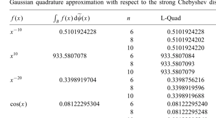
Table 1 gives quadrature results and the relative errors for a few selected functions, using a= 1, b= 2. The rst function, f(x) =x−10∈R
Table 1
Gaussian quadrature approximation with respect to the strong Chebyshev distribution (L-Quad)
f(x) RBf(x) de(x) n L-Quad Rel. error
x−10 0.5101924228 6 0.5101924228 0
8 0.5101924202 0:51·10−8
10 0.5101924220 0:16·10−8
x10 933.5807078 6 933.5807084 0:64·10−9
8 933.5807093 0:16·10−8
10 933.5807079 0:11·10−9 x−20 0.3398919704 6 0.3398756216 0:481·10−4
8 0.3398919596 0:318·10−7
10 0.3398919688 0:47·10−8
cos(x) 0.08122295304 6 0.08122295240 0:79·10−8
8 0.08122295248 0:69·10−8
10 0.08122295268 0:44·10−8
ln(x2) 2.547612410 6 2.547612416 0:24·10−8
8 2.547612413 0:12·10−8
10 2.547612411 0:39·10−9
to be at least 5. The second function, f(x) =x10, has L-degree 20 and so we need an index of at least n= 6 for exact quadrature. The third function, f(x) =x−20, has L-degree of 39, and hence an index of at least n= 10 is required for exact quadrature. Thus, the quadrature for n= 6;8 and 10 should be exact for the rst two functions, and also for f(x) =x−20 when n= 10. Recalling that 10 digits of accuracy in the computations were used, we infer from Table 1 that the error in the Laurent quadrature approximation is primarily due to round-o. It is interesting to note that for the last two functions, cos(x) and ln(x2), the quadrature rules also perform reasonably well. For related strong Chebyshev quadrature results, see [21, 22, 24, 26].
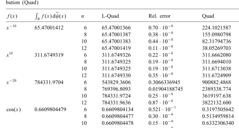
3.2. The strong Hermite distribution
The strong Hermite distribution,
de(x) = e2=2e−(x2+(2=x2))=2dx; x
∈B≡R\ {0};
is obtained by using the Transformation Theorem 1.2 on the classical Hermite distribution function d (x) = e−x2dx, x∈R. A similar formulation for the strong distribution appears in [25], with
de(x) = e−(x2+(2=x2))=2dx: (6)
For comparison purposes, we can obtain approximate integration with respect to both the classical and strong Hermite distributions. For the Laurent setting (L-Quad),
Z
B
f(x)e2=2e−(x2+(2=x2))=2dx ≈ X
k=1;:::; n;∗=±
Table 2
Gaussian quadrature approximation with respect to the strong Hermite distribution (L-Quad) and classical Hermite distri-bution (Quad)
f(x) RBf(x) de(x) n L-Quad Rel. error Quad Rel. error
x−10 65.47001412 6 65.47001366 0:70·10−8 224.1021587 2.422974040
8 65.47001387 0:38·10−8 155.0980798 1.368994140
10 65.47001383 0:44·10−8 82.31794736 0.2573381641
12 65.47001419 0:11·10−8
38.05269703 0.4187767096
x10 311.6749319 6 311.6749326 0:22·10−8 311.6662080 0:279903·10−4
8 311.6749325 0:19·10−8 311.6694010 0:177457·10−4
10 311.6749325 0:19·10−8
311.6713038 0:116407·10−4
12 311.6749330 0:35·10−8 311.6724909 0:78319·10−5 x−20 784331.9704 6 543829.3606 0.3066336945 900882.4868 0.1485984517
8 769396.8093 0.01904188745 2389338.774 2.046336073 10 784331.9724 0:25·10−8 3619197.638 3.614369648
12 784331.9636 0:87·10−8 3822132.600 3.873105706
cos(x) 0.6609804479 6 0.6609804134 0:521·10−7
0.3197505642 0.5162480748 8 0.6609804477 0:30·10−9 0.5134959814 0.2231298474
10 0.6609804478 0:15·10−9 0.6332306340 0.0419828060
12 0.6609804473 0:91·10−9
0.6922145991 0.04725427401 ln(x2) 0.3657381418 6 0.3659050839 0:4564525·10−3 0.7705753502 1.106904537
8 0.3657586794 0:561538·10−4 0.6788624452 0.8561434196
10 0.3657413394 0:87429·10−5
0.5365187768 0.4669478391 12 0.3657387335 0:16178·10−5 0.4276173519 0.1691899286
Rewriting the integrand, we obtain an equivalent expression with respect to the classical Hermite distribution (Quad):
Z
B
f(x)e(2−(2=x2))=2e−x2=2dx
≈
n X
k=1
f(xn; k)e(2−
2
=x2n; k)= 2
An; k:
Table 3
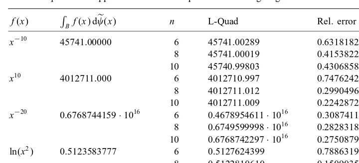
Gaussian quadrature approximation with respect to the strong Laguerre distribution
f(x) RBf(x) de(x) n L-Quad Rel. error
x−10 45741.00000 6 45741.00289 0:6318182812·10−7
8 45741.00019 0:4153822610·10−8
10 45740.99803 0:4306858180·10−7 x10 4012711.000 6 4012710.997 0:7476242371·10−9
8 4012711.012 0:2990496948·10−8
10 4012711.009 0:2242872711·10−8 x−20 0:6768744159·1016 6 0:4678954611·1016 0.3087411045
8 0:6749599998·1016 0:2828318009·10−2
10 0:6768742297·1016 0:2750879567·10−6
ln(x2) 0.5123583777 6 0.5127624399 0:7886319763·10−3
8 0.5122810610 0:1509035538·10−3
10 0.5123303897 0:5462582680·10−4 3.3. The strong Laguerre distribution
An example of a nonsymmetric SMDF is the strong Laguerre distribution,
de(x) =
1
x−
x
e−(1=)(x−(=x))dx; x∈B≡(−√;0)∪(√;∞);
obtained by using the Transformation Theorem 1.2 on the classical Laguerre distribution function d (x) =xe−xdx, x∈(0;∞). In the classical setting, is frequently taken to be 0, which is the case
we will examine here. A similar formulation for the strong distribution appears in [13, 25], with de(x) =x−1=2e−(x+2=x)=2
dx. Note that this form of the strong Laguerre distribution can be obtained by substituting u=x1=2 for x ¿0 into the associated strong Hermite distribution (6), as discussed in [13, 25].
Table 3 gives quadrature results and the relative errors for a few selected functions, using ==1. As with the previous two distributions, the Laurent quadrature for x−10 and x10 should be exact for each value of n, and also for x−20 in the case n= 10. However, for x−10 there appears to be slightly more error than anticipated from roundo. The accuracy improves for the next function, x10. For the functions x−20 and ln(x2), the quadrature approximations are only somewhat accurate, even in the best case, n= 10.
References
[1] M. Abramowitz, I.A. Stegun (Eds.), Handbook of Mathematical Functions with Formulas, Graphs and Mathematical Tables, Dover, New York, 1970.
[2] A. Bultheel, C. Diaz-Mendoza, P. Gonzalez-Vera, R. Orive, Quadrature on the half line and two point Pade approximants to Stieltjes functions. Part I. Algebraic aspects, J. Comput. Appl. Math. 65 (1995) 57–72.
[3] A. Bultheel, C. Diaz-Mendoza, P. Gonzalez-Vera, R. Orive, Quadrature on the half line and two point Pade approximants to Stieltjes functions – II: covergence, J. Comput. Appl. Math. 77 (1997) 53–76.
[5] R. Burden, J. Faires, Numerical Analysis, PWS, Kent, 1989.
[6] T.S. Chihara, An Introduction to Orthogonal Polynomials, Gordon and Breach, New York, 1978.
[7] L. Cochran, Orthogonal Laurent polynomials with an emphasis on the symmetric case, Ph.D. Thesis, Washington State University, 1993.
[8] L. Cochran, S. Clement Cooper, Orthogonal Laurent polynomials on the real line, in: S.C. Cooper, W.J. Thron (Eds.), Continued Fractions and Orthogonal Functions: Theory and Applications, Proceedings, Loen, Norway, 1992, Lecture Notes in Pure and Applied Mathematics, Marcel Dekker, New York, 1993, pp. 47–100.
[9] S.C. Cooper, P. Gustafson, The strong Chebyshev distribution and orthogonal Laurent polynomials, J. Approx. Theory 92 (3) (1998) 361–378.
[10] S.C. Cooper, P. Gustafson, Spectral analysis of the strong Tchebyche distribution, Proceedings, Conference on Applied Mathematics, University of Central Oklahoma, Edmond, OK, 1995.
[11] G. Freud, Orthogonal Polynomials, Pergamon Press, New York, 1971.
[12] P. Gustafson, Determinacy of strong moment functionals with bounded true interval of orthogonality, Ph.D. Thesis, Washington State University, 1994.
[13] B.A. Hagler, A transformation of orthogonal polynomial sequences into orthogonal Laurent polynomial sequences, Ph.D. Thesis, University of Colorado, Boulder, 1997.
[14] B.A. Hagler, W.B. Jones, W.J. Thron, Orthogonal Laurent polynomials of the Jacobi, Hermite, and Laguerre Types, Orthogonal Functions, Moment Theory, and Continued Fractions, Theory and Applications, in: William B. Jones, A. Sri Ranga (Eds.), Orthogonal Laurent Polynomials of the Jacobi, Hermite, and Laguerre Types, Lecture Notes in Pure and Applied Mathematics Series/199, Marcel Dekker, New York, 1998.
[15] W.B. Jones, O. Njastad, W.J. Thron, Two-point Pade expansions for a family of analytic functions, J. Comput. Appl. Math. 9 (1983) 105–123.
[16] W.B. Jones, O. Njastad, W.J. Thron, Orthogonal Laurent polynomials and the strong hamburger moment problem, J. Math. Anal. Appl. 98 (1984) 528–554.
[17] W.B. Jones, W.J. Thron, Orthogonal Laurent polynomials and gaussian quadrature, in: K.E. Gustafson, W.P. Reinhardt (Eds.), Quantum Mechanics in Mathematics, Chemistry, and Physics, Plenum Press, New York, 1981, pp. 449 – 445.
[18] W.B. Jones, W.J. Thron, Survey of continued fraction methods of solving moment problems and related topics, in: W.B. Jones, W.J. Thron, H. Waadeland (Eds.), Analytic Theory of Continued Fractions, Proceedings Loen, Norway, 1981, Lecture Notes in Mathematics, vol. 932, Springer, Berlin, 1982, pp. 4 –37.
[19] W.B. Jones, W.J. Thron, H. Waadeland, A strong Stieltjes moment problem, Trans. AMS 261 (1980) 503–528. [20] O. Njastad, W.J. Thron, The theory of sequences of orthogonal L-polynomials, Det Kongelige Norske Videnskabers
Selskab 1 (1983) 54–91.
[21] A. Sri Ranga, Another quadrature of highest degree of precision, Numer. Math. 68 (1994) 283–294.
[22] A. Sri Ranga, Symmetric orthogonal polyomials and the associated orthogonal L-polynomials, Proc. Amer. Math. Soc. 123 (10) (1995) 3135 –3141.
[23] A. Sri Ranga, Companion orthogonal polyomials, J. Comput. Appl. Math. 75 (1996) 23–33.
[24] A. Sri Ranga, E.X.L. de Andrade, G.M. Phillips, Associated symmetric quadrature rules, J. Comput. Appl. Math. 21 (1996) 175 –183.
[25] A. Sri Ranga, J.H. McCabe, On the extensions of some classical distributions, Proc. Edinburgh Math. Soc. 34 (1991) 19 –29.
[26] A. Sri Ranga, M. Veiga, A Chebyshev-type quadrature rules with some interesting properties, J. Comput. Appl. Math. 51 (1994) 263–265.