www.elsevier.nl/locate/cam
Product expansion for stochastic jump diusions and its
application to numerical approximation
X.Q. Liua;b, C.W. Lia;∗;1
aDepartment of Mathematics, City University of Hong Kong, 83 Tat Chee Avenue, Kowloon, Hong Kong
b
Institute of Applied Mathematics, Academia Sinica, Beijing 100080, People’s Republic of China
Received 13 March 1998; received in revised form 1 February 1999
Abstract
We derive a product expansion of the exponential Lie series in terms of a Philip Hall basis for the Chen series corresponding to the stochastic jump diusion as in Sussmann (in: C.I. Byrnes and A. Lindquist (Eds.), Theory and Applications of Nonlinear Control Systems, North-Holland, Amsterdam, 1986, pp. 323–335) for the deterministic case. Based on the expansion, we establish the Stratonovich–Taylor–Hall (STH) schemes such that each scheme involves only the minimum number of multiple stochastic integrals, which can be regarded as systems of stochastic dierential equations and approximated by a lower order scheme with an appropriate step size to ensure the necessary accuracy. Mean-square convergence of the STH schemes is shown and numerical examples are provided to illustrate the results. c1999 Elsevier Science B.V. All rights reserved.
MSC:primary 65U05; secondary 60H10; 60J65; 60G55; 41A58
Keywords:Jump diusion; Multiple stochastic integral; Stratonovich-Taylor expansion; Exponential Lie series; Philip Hall basis; Shue product; Mean square convergence
1. Introduction
Sussmann [18] expresses the Chen series as the innite product of the exponential Lie series in terms of a Philip Hall basis for the Lie algebra generated by the ordinary dierential operators, so that we can obtain numerical schemes of an appropriate order by truncating up to a certain
∗Corresponding author.
1Research supported in part by HKRGC grant CPHK 232
=93E.
number of terms of the exponential Lie series. This approach can be extended to the diusion case as in [8,19]. In this paper, we would like to develop a new product expansion of the exponential Lie series for jump diusions with a single Poisson noise while that with multi-Poisson noises is expressed as shue products which implicitly represent the ordinary part of products of multiple stochastic integrals. The algebraic structure of such type of multiple stochastic integrals with respect to Brownian motions and Poisson processes is investigated in Li and Liu [7]. In this way, we can construct the Stratonovich–Taylor–Hall (STH) schemes which are more ecient than those Stratonovich–Taylor (ST) schemes as they involve only the minimum numbers of multiple stochastic integrals, which can be regarded as systems of stochastic jump-diusion equations and approximated by a lower order scheme with an appropriate step size to ensure necessary accuracy.
The asymptotic expansion of the exponential Lie series was developed in [1,2,5] while Castell and Gaines [3] adopted this approach to substitute all the necessary multiple stochastic integrals by their conditional expectation on the partition -eld of the Brownian motions and solved the resulting ordinary dierential equations. Newton [12–14] established various asymptotically ecient schemes as to minimize the leading mean-square errors in the power series of the step size. For the survey of the numerical solution of the stochastic diusion equations, see [15,20] as well as [6,11].
Platen [16] developed Stratonovich–Taylor schemes for jump diusions while Maghsoodi and Harris [9] treated the one dimensional case and only attained lower order convergence in proba-bility since no high order multiple stochastic integrals were considered. The weak stochastic-Taylor schemes were adopted in [10] and the rate of convergence of the weak Euler scheme was investigated in Protter and Talay [17] for stochastic dierential equations (SDEs) driven by a Levy process.
Let (;F; P) be the underlying complete probability space and{Ft; t¿0}be a nondecreasing right continuous family of complete sub--algebras of F. Consider a d-dimensional stochastic dierential equation of the jump-diusion type
Xt=X0+
Z t
t0
a(s; Xs) ds+ m
X
i=1
Z t
t0
bi(s; X
s)◦ dWsi+ p
X
i=1
Z t
t0
ci(s; X
s−) dNsi (1.1)
with initial value X0: Wt = (Wt1; : : : ; Wtm) is a standard m-dimensional Ft-adapted Brownian motion
andN1 t; : : : ; N
p
t are independentFt-adapted Poisson processes with intensities1; : : : ; p, respectively,
so that {N˜it =Ni
t −it} are Ft-martingale. We assume Wt and Nt= (Nt1; : : : ; N p
t ) are independent
with zero probability of simultaneous jumps. Here ◦ denotes the Stratonovich calculus. a; bi and
cj are non-random d-dimensional vector functions with sucient smoothness. Suppose further that
ak(t; x); bk; i(t; x); ck; j(t; x); k= 1; : : : ; d; i= 1; : : : ; m; j= 1; : : : ; p; satisfy the Lipschitz and the linear
growth conditions in x so that Eq. (1.1) has the unique solution on [t0; T].
Let ={−p; : : : ;−1;0;1; : : : ; m}; M={= (1; : : : ; l): i ∈ ; l¿0} and stands for the empty
index. For ∈M; || denotes the length of ;kk=||+ number of zero component of ; − and
− denote the remainder indices by deleting respectively the rst and the last component of if ||¿1. For a square integrable Ft-adapted process ft, dene the multiple Stratonovich integrals J by J[f];=f and
J[f];=
Z
· · ·
Z s2−
fs1−dZ 1 s1 · · ·dZ
l
sl;
where dZi
s = dNs−i; i ¡0; dZs0= ds and dZsi=◦dWsi; i ¿0: For brevity, denote J[1]; by J; ; or
Let the operators associated with the system (1.1) be L−if(t; x) =f(t; x+ci(t; x))−f(t; x); i= 1; : : : ; p;
L0f(t; x) =
@f @t(t; x) +
d
X
k=1
ak(t; x)@f
@xk(t; x);
Lif(t; x) = d
X
k=1
bk; i(t; x)@f
@xk(t; x); i= 1; : : : ; m:
(1.2)
Denote L=id, the identity operator, and L=L1L2· · ·Ll:The Stratonovich–Taylor expansion for the exact solution Xt of the jump diusions can be derived by the Ito’s rule, see [16].
Theorem 1.1. For any stopping times andsuch thatt06 ¡ 6T a.s.; we have
X=X+
X
∈Ar
J; ; L(; X) +
X
∈R(Ar)
J[L(·; X:)]; a:s:; (1.3)
whereAr={∈M:kk62r}; R(Ar) ={∈M\Ar:−∈Ar} and is the identical mapping on
Rd.
The Stratonovich–Taylor (ST) scheme of an integer order r is thus
Yn+1=
X
∈Ar
J; tn; tn+1L(tn; Yn) (1.4)
while the ST scheme of a half-integer order r is
Yn+1=
X
∈Ar
J; tn; tn+1L(tn; Yn) + (L I 0)r
+0:5(t
n; Yn)(tn+1−tn)r+0:5=(r+ 0:5)!; (1.5)
where
LI
0=L0+
1 2
m
X
j=1
L2
j: (1.6)
The corresponding operator of Eq. (1.4) can be expressed by truncating up to an order r the Chen series
S;=
X
∈M
J; ; L; 06t0666T; (1.7)
with respect to the Brownian motion W and the Poisson process N over [; ].
2. Philip Hall basis
Let Br(L−p; : : : ; Lm) be the set of the formal brackets of L−p; : : : ; Lm with Lie bracket [A; B] =AB−
BA andM be the corresponding index set of the formal brackets of :Denote L[; ]= [L; L]; ; ∈ M: Similarly we can dene the degree||and kk as those indices in M. Let MH⊂M be a Philip Hall set with the order 4 such that −p≺ · · · ≺ −1≺0≺1≺ · · · ≺m and
(a) ⊂M
H;
(c) [; ]∈MH if and only if (i) ≺; ; ∈MH; (ii) either ||= 1 or = [; ] with ; ∈MH and 4: It is known that L
H ={L:∈MH} forms an algebraic basis of the Lie algebra L(L−p; : : : ; Lm):
Here is a Philip Hall basis MH=S
i¿1M (i)
H with a total order 4 and M (i)
H consists of elements of
degree i. (a) M(1)
H = ;j14j2 if j16j2:
(b) M(2)
H ={[j1; j2]:j1¡ j2; j1; j2 ∈ }; [j1; j2]4[j3; j4] if j1j26j3j4:
(c) M(3)
H ={[j1;[j2; j3]]: j26j1; j1 ∈ ;[j2; j3]∈M (2) H };
[j1;[j2; j3]]4[j4;[j5; j6]] if j1j2j36j4j5j6:
(d) M(4;1)
H ={[j1;[j2;[j3; j4]]]: j26j1; j1∈ ; [j2;[j3; j4]]∈M(3)H };
[j1;[j2;[j3; j4]]]4[j5;[j6;[j7; j8]]] if j1j2j3j46j5j6j7j8:
M(4;2)
H ={[[j1; j2];[j3; j4]]: j1j2¡ j3j4;[j1; j2];[j3; j4]∈M(2)H };
[[j1; j2];[j3; j4]]4[[j5; j6];[j7; j8]] if j1j2j3j46j5j6j7j8:
M(4)
H =M (4;1) H ∪M
(4;2)
H ; ≺ if ∈M (4;1)
H ; ∈M (4;2) H :
(e) M(5;1)
H ={[j1;[j2;[j3;[j4; j5]]]]: j26j1; j1 ∈ ;[j2;[j3;[j4; j5]]]∈M(4H;1)};
[j1;[j2;[j3;[j4; j5]]]]4[j6;[j7;[j8;[j9; j10]]]] if j1j2j3j4j5 6j6j7j8j9j10:
M(5;2)
H ={[[j1; j2];[j3;[j4; j5]]]: [j1; j2]∈M (2)
H ;[j3;[j4; j5;]]∈M (3) H };
[[j1; j2];[j3[j4; j5]]]4[[j6; j7];[j8[j9; j10]]] if j1j2j3j4j56j6j7j8j9j10:
M(5)
H =M (5;1) H ∪M
(5;2)
H ; ≺ if ∈B(5;1); ∈B(5;2):
Note that j1j2· · ·jl denotes the integer Plk=1ml
−kj
k as a (p+m+ 1) adic number if all ji¿0:
For ||¿1; can be expressed uniquely as ad(1)j(2) with |2|= 1 or 2= [3; 4]; 3 ≺1:
Therefore we can dene the stochastic integral C; ; =
R
c; ; t where c; ; t is dened recursively by
c; ; t=j1!Cj1; ; t−c2; ; t with ck; ; t= dZ k t:
3. Product expansion of exponential Lie series
We will extend the result in Sussmann [18] to express the Chen series as an innite product of the exponential Lie series to jump diusions. For the single Poisson noise case, the expression is more explicit while for the multi-Poisson noise case, the expression is more complicated and is in terms of shue products.
3.1. The single Poisson noise case (p= 1)
Let
e
Lk=
ln(1 +L
−1); k=−1;
Lk; k= 0; : : : ; m
(3.1)
and the product of the exponential Lie series in terms of a Philip Hall basis be
P;=
← Y
∈MH
The arrow indicates the order of the factors appearing from the right to the left according to 4. We state the following adjoint representation of Lie algebra without proof.
Lemma 3.1. For A and B in a Lie algebra; we have the following adjoint representation:
eABe−A=B+[A; B] 1! +
[A;[A; B]]
2! +· · ·= ∞ X
k=0
(ad(A))k(B)=k!:
The following theorem is the extension of the result in [18] to the jump-diusion case, see also [8,19] for the diusion case.
Theorem 3.2. The Chen series has a product expansion of the exponential Lie series of the form
(3:2);i.e. S;=P;:
Proof. Let {1; 2; : : :} be the indices in MH ordered by 4. Dene G0 = {1; 2; : : : ; m+2} =
{−1;0; : : : ; m} and Gj ={(adj)k(): ∈ Gj−1\{j}; k¿0}; j¿1: Let S; t1 =S; t: It follows from
the denition of S; t that dS; t1 =S; t1
P
∈G0c;;tL: LetS 2
; t=S; t1 exp(−C−1;;teL−1): Applying the Ito’s
rule, we have
dS; t2 =S; t1 X
∈G0\{−1}
c;;tLexp(−C−1;;tLe−1) +{(S; t1 −+S
1 ; t−L−1)
×exp(−C−1;;t−
e
L−1−Le−1)−S; t1 −exp(−C−1;;t−Le−1)}dNt1
=S; t1 X
∈G0\{−1}
c;;tLexp(−C−1;;tLe−1)
+S1
; t−{(1 +L−1)exp(−Le−1)−1}exp(−C−1;;t−eL−1)dNt1
=S2
; texp(C−1;;teL−1)
X
∈G0\{−1}
c;;tLexp(−C−1;;tLe−1)
=S2 ; t
X
∈G1
c;;tLe
by the adjoint representation. For k¿2, assume dSk
; t=S k ; t
X
∈Gk−1
c;;tLe (3.3)
and let Sk+1
; t =S; tk exp(−Ck;;tLek): Since Ck;;t; k¿2; are continuous, dS; tk+1=S; tk X
∈Gk−1
c;;tLeexp(−Ck;;tLek)−S
k
; tck;;tLekexp(−Ck;;teLk)
=S; tk+1exp(Ck;;teLk) X
∈Gk−1\{k}
c;;tLeexp(−Ck;;tLek)
=S; tk+1 X
∈Gk
by the adjoint representation. We have Eq. (3.3) for k¿2 by induction. Thus Sk
Let r denote the truncation up to the indices in Ar and
∗r =
wheretn=tn+1−tn:Then the Stratonovich–Taylor–Hall (STH) scheme of an integer or a half-integer
order r is
given Philip Hall basis is given as follows:
−1
2
m
X
j=1
Wnj(Nn1)2LjL3−1+
11 24(N
1 n)
2L4
−1−
1 4(N
1 n)
3L4
−1
−1
2 X
j1¿0; j26=0
{Zj2
n C[−1; j1]; n[L2−1; Lj1]Lj2+C[j2;[−1; j1]]; n[Lj2;[L 2
−1; Lj1]]}
−1
2C[−1;0]; n[L
2
−1; L0] +
1 3
m
X
j=1
C[−1; j]; n[L3−1; Lj]: (3.8)
Note. All the summation indices are excluded from zero.
3.2. The multi-Poisson noise case (p ¿1)
In general the product expansion of the exponential Lie series for the Chen series is very com-plicated and cannot be expressed in terms of ˜L as in Eq. (3.2). However, the Chen series can be expressed as shue products of the exponential Lie series. The algebraic structure of multiple stochastic integrals related to shue products is illustrated in Li and Liu [7].
For = (1; : : : ; l) and = (1; : : : ; k) in M, dene the shue product
J? J= (J−? J)◦J(l)+ (J? J−)◦J(k);
where J ◦J =J and denotes the concatenation of and . Then the shue product is
commutative and associative. The usual product JJ=J? J+J♦J
is decomposed into the shue product and the ♦ product
J♦J= l
X
i=1 k
X
j=1
i;j(JLiJjL)◦J(i)◦(JRi ? JRj);
where i; j= 1; i=j ¡0 and i; j= 0 otherwise; Li and Ri are, respectively, the left and right indices
of the component i such that =Li(i)Ri: Observe that the shue product contains those terms
of the degree ||+|| while the ♦ product involves those terms of lower degree. Thus for ∈M; there exist two nite subsets F1; F2⊂M such that
C=
X
∈F1
aJ+
X
∈F2
aJ;
where ||=||; ∈F1 and ||¡||; ∈F2; a ∈Q. Denote C?=
P
∈F1 aJ; the principal part
of C; i.e., we may regard c?j symbolically as the ordinary part of the dierential operatorcj so that
c?
j ’s comply with the ordinary dierential rule. From [18], we have the following result.
Theorem 3.3. The Chen series has a shue product expansion of the exponential Lie series in terms of a Philip Hall basis
S;=P;,
←?
Y
∈MH
exp?(C?
; ; L); (3.9)
The STH schemes of an integer or a half-integer order is still expressed as Eq. (3.4). After expanding the right-hand side of Eq. (3.9), the truncation becomes
r(Pn) =id+
the degree 4 in terms of the usual products as follows:
Zj1? C?
Remark. All the other forms of shue products of degrees less than or equal to 4 will be the same as the usual products. Eqs. (3:5)–(3:8) may also be obtained from Eq. (3:10) with p= 1
using the above shue product relation.
4. Mean-square convergence
The evaluation of multiple stochastic integrals is necessary to obtain a high order approximation. For the diusion case, Milstein [11], Kloeden and Platen [6] suggest the Fourier series approach while Gaines and Lyons [4] apply the Marsaglia rectangle-wedge-tail method to generate stochastic area Ito integrals which is not easy to generalize in higher dimensions.
In order to refer to the common interval [0;1] of the integration, we make the change of variables
on [0; j(−)]. Thus
J; ; = (−)kbk=2J;V0;1; (4.2)
C; ; = (−)kbk=2C;V0;1; (4.3)
wherebdenotes the remainder index by deleting all negative components;JV
andCV are the multiple
stochastic integrals with respect to V as J and C with respect to Z. We will regard Eqs. (4.2) and
(4.3) as systems of stochastic dierential equations and solve them by the STH0.5 (Euler) scheme with a maximum step size h=2r+1−kbk or 2r+1−kbk on [0;1] so as to have an order r convergence.
Theorem 4.1 (r=integer or half-integer). Let Yn be the approximate solution obtained by Eqs.
(1:4); (1:5) or (3:4) and Xn be the exact solution of (1:1) at tn; respectively. Suppose all the
partial derivatives of ak(t; x); bk; i(t; x) andck; j(t; x) with respect to t up to order r or r+ 0:5 if r is
a half-integer and x up to order 2r+ 1 respectively are continuous and locally bounded in x∈Rd
and each t ∈[t0; T]; ak(t; x); bk; i(t; x) and ck; j(t; x) are at most of locally linear growth in x ∈Rd for each t ∈[t0; T]: If E{kX0−Y0k
2
|F
t0}=O(
2r) and all necessary multiple stochastic integrals
J or C are approximated by the STH0.5 scheme with a maximum step size h=2r+1−kbk or
2r+1−kbk on [0;1]; then
(E{kXn−Ynk 2
|F
t0})
1=26C(r; T; d; X
0)r (4.4)
locally up to n6T= for some constant C(r; T; d; X0):
Proof. It is not hard to show by induction for some constant C() the following estimate:
E{|J[g];| 2|F
t0}6C()
(−)kk−1Z
E{|gs|2|Ft0}ds
+ ˜1;0(−)
kkZ
E{|L1gs| 2|F
t0}ds
; (4.5)
where ˜1;0 = 1; 1¿0 and ˜1;0= 0 otherwise. Repeatedly applying Eq. (4.5), we have the
sec-ond moment estimate of all multiple stochastic integrals in the scheme. The rest of the proof is straightforward and is similar to the diusion case.
5. Numerical implementation
Example 5.1. Consider the following stochastic Ginzburg–Landau equation driven by a jump-diusion noise
dXt= (−Xt3+Xt=2) dt+Xt◦dWt+XtdNt (5.1)
with the exact solution
Xt=
X0exp{t=2 +Wt+ (ln 2)Nt}
(1 + 2X2 0
Rt
0exp(s+ 2Ws+ 2(ln 2)Ns) ds)1=2
: (5.2)
The STH0.5, ST1.0, STH1.0, ST1.5 and STH1.5 schemes for (5.1) are, respectively, as follows:
Yn+1=Yn+ (−Yn3+Yn)tn+YnWn+YnNn; (5.3)
Yn+1=Yn+ (−Yn3+Yn=2)tn+YnWn+YnNn
+Yn{J(−1;−1); n+J(−1;1); n+J(1;−1); n+J(1;1); n}; (5.4)
Yn+1=Yn+ (−Yn3+Yn=2)tn+YnWn+YnNn
+Yn{(Nn)2=2−Nn=2 +WnNn+ (Wn)2=2}; (5.5)
Yn+1=Yn+ (−Yn3+Yn=2)tn+YnWn+YnNn
+Yn{J(−1;−1); n+J(−1;1); n+J(1;−1); n+J(1;1); n}
+ (−Yn3+Yn=2)J(0;−1); n+ (−7Yn3+Yn=2)J(−1;0); n
+ (−Y3
n +Yn=2)J(0;1); n+ (−3Yn3+Yn=2)J(1;0); n
+Yn{J(−1;−1;−1); n+J(−1;−1;1); n+J(−1;1;−1); n+J(1;−1;−1); n
+J(−1;1;1); n+J(1;−1;1); n+J(1;1;−1); n+J(1;1;1); n}
+ (3Y5
n −7Yn3+Yn)(tn)2=2; (5.6)
Yn+1=Yn+ (−Yn3+Yn=2)tn+YnWn+YnNn
+Yn{(Nn)2=2−Nn=2 +WnNn+ (Wn)2=2}
+ (−Y3
n +Yn=2)tnNn−6Yn3C[−1;0]
+ (−3Yn3+Yn=2)tnWn+ 2Yn3C[0;1]
+Yn{(Nn)3=6−(Nn)2=2 +Nn=3 +Wn(Nn)2=2
+Nn(Wn)2=2−WnNn=2 + (Wn)3=6}
+ (3Yn5−7Yn3+Yn)(tn)2=2: (5.7)
The schemes ST1.0 and ST1.5 involve, respectively, 4 and 16 distinct multiple stochastic integrals to be approximated while the schemes STH1.0 and STH1.5 involve respectively 0 and 2 distinct multiple stochastic integrals so that the STH schemes will save more computing time than those ST schemes particularly for high order schemes.
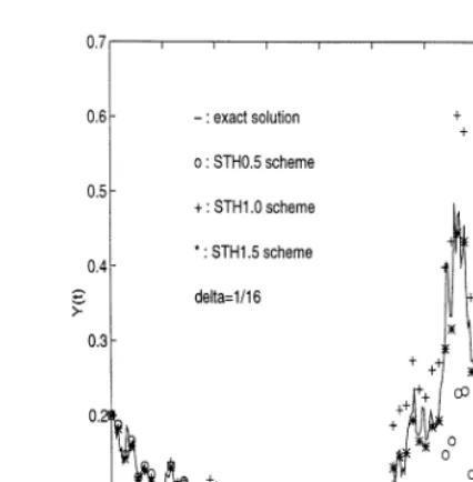
In Fig. 1, we plot the approximations using the STH schemes of the order 0.5, 1.0 and 1.5, respectively, with the step size = 2−4 and the exact solutionX of Eq. (5.2) along a Brownian path
Fig. 1. Exact solution and approximations by STH schemes with = 2−4 .
Table 1
P|
(X5:0−YK)=X5:0|=1000
−log2() STH0.5 ST1.0 STH1.0 ST1.5 STH1.5
2 1.117858 0.991177 0.966794 1.376278 0.214447
3 0.618411 0.501596 0.489133 0.466588 0.062548
4 0.479329 0.221514 0.213749 0.217543 0.027051
5 0.291707 0.117271 0.112393 0.103632 0.010045
6 0.211376 0.062888 0.063115 0.048818 0.003647
7 0.148874 0.028506 0.028493 0.022386 0.001069
8 0.071621 0.014376 0.014648 0.012075 0.000327
9 0.062520 0.007904 0.008191 0.005500 0.000128
well after t= 3 and the result using the high order STH1.5 scheme appears much better even for a coarse step size.
In Table 1, we list the relative average error of 1000 approximate solutions YK; K=5:0= atT=5:0
using various ST and STH schemes with step sizes ranging from 2−2 to 2−9:The step size should
be rened for lower order schemes to maintain the same accuracy as that for higher order schemes. For instance, to obtain a relative average accuracy of one decimal place, the step size for schemes STH0.5, STH1.0 (ST1.0) and STH1.5 (ST1.5) are at most 2−9;2−6(2−6) and 2−3(2−6), respectively.
are less than those of the ST schemes. This is due to the fact that the number of multiple stochastic integrals is reduced to the minimum in the STH schemes.
Example 5.2. Consider the following two-dimensional system of jump diusion. dX1
t =X 1 t ◦dW
1 t +X
2 t ◦dW
2 t +X
2 t−dNt1;
dXt2=Xt2◦dWt1+Xt1−dNt2: (5.8) The STH0.5, ST1.0, STH1.0, ST1.5 and STH1.5 are, respectively, as follows.
Yn1+1=Yn1(1 +Wn1+tn=2) +Yn2(W 2 n +N
1
n); (5.9)
Yn2+1=Yn1Nn2+Yn2(1 +Wn1+tn=2);
Y1 n+1=Y
1
n{1 +W 1
n +J(1;1); n+J(−2;−1); n+J(−2;2); n}
+Y2
n{Wn2+Nn2+J(2;1); n+J(−1;1); n+J(1;2); n+J(1;−1); n}; (5.10)
Yn2+1=Yn1{Nn1+J(−2;1); n+J(1;−2); n}
+Yn2{1 +Wn1+J(1;1); n+J(2;−2); n+J(−1;−2); n};
Y1
n+1=Yn1{1 +W 1
n + (W 1 n)
2=2 +C
[−2;−1]; n+C[−2;2]; n}
+Yn2{Nn2+Wn2+Nn1Wn1+Wn1Wn2}; (5.11)
Yn2+1=Yn1{Nn1+Nn2Wn1}+Yn2{1 +Wn1+Nn2Wn2+Nn2Nn1 +(W1
n)
2=2−C
[−2;−1]; n−C[−2;2]; n−C[−1;2]; n};
Yn1+1=Yn1{1 +Wn1+J(1;1); n+J(−2;−1); n+J(−2;2); n+J(1;1;1); n
+J(−2;2;1); n+J(−2;1;2); n+J(−2;−1;1); n+J(1;−2;2); n
+J(−2;1;−1); n+J(1;−2;−1); n+ (tn)2=8}
+Yn2{Wn2+Nn2+J(2;1); n+J(−1;1); n+J(1;2); n+J(1;−1); n
+J(2;−2;2); n+J(−1;1;1); n+J(1;2;1); n+J(1;−1;1); n+J(1;1;−1); n
+J(2;1;1); n+J(1;1;2); n+J(−1;−2;2); n+J(2;−2;−1); n+J(−1;−2;−1); n}; (5.12)
Yn2+1=Yn1{Nn1+J(−2;1); n+J(1;−2); n+J(−2;1;1); n+J(1;−2;1); n
+J(1;1;−2); n+J(−2;2;−2); n+J(−2;−1;−2); n}
+Yn2{1 +Wn1+J(−1;−2); n+J(2;−2); n+J(1;1); n+J(1;1;1); n
+J(2;−2;1); n+J(−1;−2;1); n+J(2;1;−2); n+J(−1;1;−2); n
+J(1;2;−2); n+J(1;−1;−2); n+ (tn)2=8};
Y1
n+1=Yn1{1 +Wn1+ (Wn1)2=2 +C[−2;−1]; n+C[−2;2]; n+ (Wn1)3=6
+Wn1C[−2;2]; n+Wn1C[−2;−1]; n+ (tn)2=8}
+Y2 n{N
1 n +W
2 n +N
1 nW
1 n +W
1 nW
2
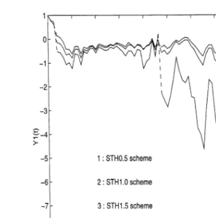
Fig. 2. Approximations of Xt1 by STH schemes with= 2−3.
−N1
nC[−2;1]; n−Nn1C[−2;2]; n+ 2C[−1;[−2;1]]; n+ 2C[2;[−2;1]]; n
+ 2C[−1;[−2;2]]; n+Wn2(Nn1)2=2−Wn2Nn1=2
+ 2C[2;[−2;2]]; n−Wn2C[−2;2]; n+Nn1(W 1 n)
2=2}; (5.13)
Y2 n+1=Y
1 n{N
2 n +N
2 nW
1 n +N
2 n(N
1 n)
2=2 +N2
nC[−2;−1]; n −2C[−2;[−2;1]]; n+Nn2C[−2;2]; n−2C[−2;[−2;2]]; n}
+Yn2{1 +Wn1+ (Wn1)2=2 +Nn2Nn1−C[−2;−1]; n
+N2 nW
2
n −C[−2;2]; n+Nn2N 1 nW
1 n −W
1
nC[−2;−1]; n
+Nn2Wn1Wn2−Wn1C[−2;2]; n+ (Wn1)
3=6 + (t n)3=8}:
The STH1.5 scheme (5.13) involves only 6 distinct multiple stochastic integrals of the degree 3 while the ST1.5 scheme (5.12) involves 28 distinct multiple stochastic integrals of the same degree. Hence the STH schemes are more ecient than those ST schemes in higher dimensions.
In Fig. 2, the approximations Y1 of the rst component of the solution X of Eq. (5.8) using
various STH schemes of the order 0.5, 1.0, 1.5 are plotted with = 2−3: The result using the
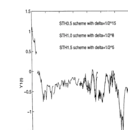
STH0.5 (Euler) scheme is completely inaccurate after time t= 4 and that using the STH1.0 scheme is still worse aftert=6 while that using the STH1.5 scheme is better when compared with the results using various STH schemes of the order 0.5, 1.0, 1.5 with step sizes = 2−15;2−8;2−5, respectively,
as shown in Fig. 3.
In Table 2, we list the average of successive errors of the rst component YK1;; K = 10:0=; at
Fig. 3. Approximations of X1
t by STH schemes with better accuracy.
Table 2
P
|YK1;−Y
1;2 K |=1000
−log2() STH0.5 ST1.0 STH1.0 ST1.5 STH1.5
3 0.034095 0.009888 0.011365 0.003482 0.003141
4 0.021090 0.005274 0.004393 0.002023 0.001150
5 0.013925 0.004660 0.004293 0.001179 0.001291
6 0.003204 0.000465 0.001396 0.000827 0.002879
7 0.001399 0.000689 0.000867 0.000190 0.000245
8 0.003110 0.000628 0.000738 0.000121 0.000270
9 0.003803 0.000297 0.000477 0.000107 0.000189
of two decimal places only while that using the STH1.0 (ST1.0) and STH1.5 (ST1.5) schemes have an accuracy of three decimal places with step sizes 62−9 and 62−7, respectively.
References
[1] G. Ben Arous, Flots et series de Taylor stochastiques, Probab. Theory Relat. Fields 81 (1989) 29–77. [2] F. Castell, Asymptotic expansion of stochastic ows, Probab. Theory Relat. Fields 96 (1993) 225–239.
[3] F. Castell, J.G. Gaines, The ordinary dierential equation approach to asymptotically ecient schemes for solution of stochastic dierential equations, Ann. Inst. H. Poincare Probab. Statist. 32 (1996) 231–250.
[4] J.G. Gaines, T.J. Lyons, Random generation of stochastic area integrals, SIAM J. Appl. Math. 54 (1994) 1132–1146. [5] Y.Z. Hu, Serie de Taylor stochastique et formule de Campbell–Hausdor, d’apres Ben Arous, in: Seminaire de
[6] P.E. Kloeden, E. Platen, Numerical Solution of Stochastic Dierential Equations, Springer, Berlin, 1992.
[7] C.W. Li, X.Q. Liu, Algebraic structure of multiple stochastic integrals with respect to Brownian motions and Poisson processes, Stochastics Stochastics Rep. 61 (1997) 107–120.
[8] X.Q. Liu, C.W. Li, Discretization of stochastic dierential equations by the product expansion for the Chen series, Stochastics Stochastics Rep. 60 (1997) 23–40.
[9] Y. Maghsoodi, C.J. Harris, In-probability approximation and simulation of nonlinear jump-diusion stochastic dierential equations, IMA J. Math. Control Inform. 4 (1987) 65–92.
[10] R. Mikulevicius, E. Platen, Time discrete Taylor approximation for Itˆo processes with jump component, Math. Nachr. 138 (1988) 93–104.
[11] G.N. Milstein, Numerical Integration of Stochastic Dierential Equations, Kluwer Academic Publishers, Dordrecht, 1995.
[12] N.J. Newton, An asymptotically ecient dierence formula for solving stochastic dierential equations, Stochastics 19 (1986) 175–206.
[13] N.J. Newton, An ecient approximation for stochastic dierential equations on the partition of symmetrical rst passage times, Stochastics Stochastics Rep. 29 (1990) 227–258.
[14] N.J. Newton, Asymptotically ecient Runge–Kutta methods for a class of Ito and Stratonovich equations, SIAM J. Appl. Math. 51 (1991) 542–567.
[15] E. Pardoux, D. Talay, Discretization and simulation of stochastic dierential equations, Acta Appl. Math. 3 (1985) 23–47.
[16] E. Platen, An approximation method for a class of Ito processes with jump component, Lietuvos Matem. Rinkinys 22 (1982) 124–136.
[17] P. Protter, D. Talay, The Euler scheme for Levy driven stochastic dierential equations, Ann. Probab. 25 (1997) 393–423.
[18] H.J. Sussmann, A product expansion for the Chen series, in: C.I. Byrnes, A. Lindquist (Eds.), Theory and Applications of Nonlinear Control Systems, North-Holland, Amsterdam, 1986, pp. 323–335.
[19] H.J. Sussmann, Product expansions of exponential Lie series and the discretization of stochastic dierential equations, in: W. Fleming, P.L. Lions (Eds.), Stochastic Dierential Systems, Stochastic Control Theory and Applications, Springer, New York, 1988, pp. 563–582.