*Corresponding author.
A two machine bicriteria scheduling problem
Subhash C. Sarin*, R. Hariharan
Department of Industrial and Systems Engineering, 250 New Engineering Building, Virginia Polytechnic Institute and State University, Blacksburg, VA 24061, USA
Received 10 June 1998; accepted 26 August 1998
Abstract
In this paper we consider the bicriteria problem of schedulingnjobs on two parallel machines to minimize the primary criterion of maximum tardiness (¹
.!9) and the secondary criterion of number of tardy jobs (NT). Algorithms are
developed to optimize each of these criteria. Some properties on which the ¹
.!9 algorithm is based are developed.
Computational experience with the algorithms is also reported. ( 2000 Elsevier Science B.V. All rights reserved.
Keywords: Bicriteria scheduling; Two machines
1. Introduction
In this paper we consider the problem of schedul-ing n jobs on two parallel machines to minimize maximum tardiness (¹
.!9) and total number of tardy jobs (NT). The former is considered as a pri-mary criterion while the latter is considered as a secondary criterion. The primary criterion is the one that is optimized "rst while the secondary criterion is optimized subject to the value obtained for the primary criterion.
A survey of the work done on the single machine bicriteria problem is given by Dileepan and Sen [1] while the two and higher machine bicriteria prob-lems have been addressed only recently. Cenna and Tabucanon [2] discuss a bicriterion parallel ma-chine problem of minimizing total #owtime and
¹
.!9. They present a procedure to generate e$cient
solutions based on an approach which "rst allo-cates jobs in accordance with a list schedule and then determines e$cient sequences on individual machines using a single machine bicriteria proced-ure. Daniels and Chambers [3] consider the se-quencing of jobs through a multimachime#owshop for the two criteria of minC
.!9(maximum comple-tion time among all machines) and¹
.!9. The aim is to develop e$cient set of solutions. An algorithm is suggested to generate an exact number of e$cient solutions for the two machine problem while heu-ristic procedures are suggested for approximating the e$cient sets for higher number of machines.
Considering only the ¹
.!9 criterion problems, Gary and Johnson [4] present a procedure for a special version of this problem in which the pro-cessing time of all the jobs is identical and jobs have arbitrary precedence among them. Townsend [5] considers thenjob,mmachine, min¹
.!9#owshop problem and suggests a branch and bound proced-ure for its solution. In their paper, Nunnikhoven and Emmons [6] develop enumerative optimization
methods to determine minimum number of parallel processors required to meet due dates. These methods can be used to minimize¹
.!9on a given number of machines by sequentially trying various tardiness values until the attainment of a minimum tardiness value for which a schedule can be found.
The two machine ¹
.!9 problem is shown to be NP-complete [7]. Hence, the bicriteria problem under consideration is also NP-complete. Conse-quently, we develop an approximate algorithm for this problem that generates almost optimal solu-tions. To that end, we "rst present some assump-tions and notation that are used in the remainder of the paper. This is followed by motivation regarding the development of the algorithms for both the criteria. Some properties on which the algorithm for minimizing ¹
.!9 is based are developed next. The algorithms are then described. In the end, some computational experience with these algorithms is presented.
2. Assumptions and notation
Considering the ¹
.!9 problem, there exists an allocation of the jobs to the two machines corre-sponding to the optimal value of¹
.!9such that the jobs on each machine are arranged in EDD order. This follows from the fact that if the jobs on each machine are not in EDD order then the¹
.!9value cannot be worsened by arranging them in EDD order. Hence, without loss of generality we assume that the jobs on each machine are arranged in EDD order. In an EDD sequence on a machine, if two Jobsiandjhave equal due dates, then the job with a higher processing time precedes the job with a lower processing time. We use the notationi.b.jto represent the fact that Job i precedes Job j in a sequence of jobs on both the machines. Converse-ly also, the notation,i.b.j. will mean thatd
i(djand ifd
i"djthenpi*pj. Also, by the notationi.b.k.b.j. we imply that Jobiprecedes Jobkand Jobk pre-cedes Job j in a sequence of jobs on both the machines. Let ¹
.!91 be the maximum tardiness
among the jobs on machine 1 and ¹
.!92 be the
maximum tardiness among the jobs on machines 2. In the sequel, we will refer to the ¹
.!9 job on Machine 1 by k and that on Machine 2 by l.
Machines 1 and 2 are labeled such thatk.b.l. The maximum tardiness value for the two machine problem, ¹
.!9"max(¹.!91,¹.!92), and the
opti-mal two machine maximum tardiness value will be denoted by ¹H
.!9. We will also use the notation
¹
i and ¸i to represent the tardiness and lateness, respectively, of a jobi, in a sequence of the jobs on the two machines.
3. Motivation regarding the development of the algorithms
The procedure that is developed to minimize
¹
.!9"rst aims at the determination of an allocation of the jobs to the two parallel machines such that the minimum of the¹
.!9values of the jobs on the two machines sets a lower bound on¹H
.!9so that it lies in the closed interval (or range) [¹
.!91,¹.!92].
This will be called the &range location phase' or Phase 1 of the algorithm. Starting from a given allocation of the jobs to the two machines, this is accomplished by exchanging them between the two machines so that no further exchange can lead to a value of maximum tardiness less than the current minimum between the ¹
.!91 and ¹.!92 values.
Single job exchanges and multiple job exchanges between the two machines are considered. All such exchanges are made depending upon the locations of the¹
.!91and¹.!92jobs on the machines. A set
of conditions are developed in Section 4 to deter-mine the jobs to switch to result in successful exchanges.
After obtaining a closed interval [¹
.!91,¹.!92]
by the process of range location, we next attempt to reduce this range so that the ¹H
.!9 value lies on a smaller interval. This will be called the &range reduction phase'or Phase II of the algorithm. Such a reduction can be performed in the following three di!erent ways: (i) by reducing the higher of the two
¹
.!9 values while keeping the other one the same (referred to as Strategy A); (ii) by reducing the higher and increasing the lower of the two values (referred to as Strategy B); (iii) by increasing the lower of the two ¹
.!9 values while keeping the other one the same (referred to as Strategy C).
Fig. 1. Overall logic of the procedure used.
between the two machines including single and multiple job exchanges. The process of considering all possible multiple job exchanges is equivalent of solving a knapsack problem. Due to an extensive amount of computational e!ort involved to do this, we consider instead exchanges of a particular type. This makes the algorithm a heuristic procedure, even though, as is shown later, the solutions obtained are found to be almost optimal. After a successful range reduction step, the range reloca-tion step is executed to see if the range can be relocated. The overall logic of the algorithm is given in Fig. 1.
The algorithm developed to minimize NT follows a search tree procedure. The scheduling of jobs is carried out beginning from the last position. Hence, the makespan value on each machine needs to be known. These makespan values are deter-mined based on the¹
.!9value and the maximum due date. Since the jobs are scheduled backward, the"nish time of a job is known when it is sched-uled, and accordingly its tardiness value can be determined. Hence, only those jobs that do meet the primary criterion at a position are considered for that position. The allocation of each eligible job there gives rise to a branch of the search tree and a corresponding node of the partial sequence.
4. Exchange procedure analysis
Before developing the conditions for the jobs to be exchanged, let us"rst illustrate the concept, on which the procedure is based, through two simple examples.
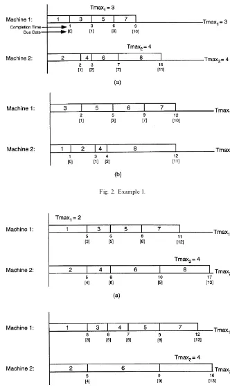
Example 1.Consider the processing time and due
date data for the eight jobs given below.
Job 1 2 3 4 5 6 7 8
Processing time 1 2 2 1 3 4 3 8
Due date 0 1 1 2 3 7 10 11
The jobs are numbered in the nondecreasing order of their due dates. They are allocated in this order to the earliest available position on the two parallel machines. The resulting schedule is shown in Fig. 2(a). In this schedule, ¹
.!91"3 and it occurs for
Job 5, while¹
.!92"4 and it occurs for Job 8. Thus, ¹
.!9"4. Now, if we remove Job 1 from Machine 1 and Job 6 from Machine 2 and put them in their EDD positions on Machines 2 and 1, respectively, the resulting schedule (shown in Fig. 2(b)) has
¹
.!9"2. Incidentally, the new ¹.!91 and ¹
.!92values happen to be the same. This need not
be the case in general. Thus, by switching some jobs between the machines, the new¹
.!9value became less than the current min(¹
.!91,¹.!92) value ("3).
This is the range relocation concept.
Example 2. Consider another example shown
below.
Job 1 2 3 4 5 6 7 8
Processing time 5 5 1 1 2 4 3 7
Due date 3 4 5 6 8 9 12 13
The starting schedule is shown in Fig. 3(a). For this schedule,¹
.!91"2 and¹.!92"4. Clearly, the ¹
.!9value for this problem cannot be less than 2 as
¹
.!91 occurs for the "rst job on Machine 1. The
range for¹
.!9is therefore [2, 4]. Now, if we shift Job 4 from Machine 2 to Machine 1, the resulting schedule (shown in Fig. 3(b)) has¹
.!92"3. Thus,
the¹
.!9 range has been reduced to [2, 3]. This is the range reduction concept. The range of¹
.!9 is reduced here by reducing¹
Fig. 2. Example 1.
Fig. 4. Exchange procedure analysis.
also be reduced by increasing¹
.!91or by
simulta-neously increasing¹
.!91and reducing¹.!92. Also,
note that, shifting Job 2 or Job 6 individually in Fig. 3(a) does not result in range reduction. However, if an appropriate job is also shifted from Machine 1 to Machine 2 then it may. For instance, if Job 6 is shifted to Machine 1 and Job 5 is shifted to Machine 2 in Fig. 3(a), then range reduction is achieved. In fact, then,¹
.!91"2 and¹.!92"2.
In general, multiple jobs from Machine 1 may be switched with multiple jobs from Machine 2 to e!ect the change with respect to both range reloca-tion and range reducreloca-tions. To see this, consider the situation in Fig. 3(b). If Job 6 from Machine 2 is switched with Jobs 4 and 5 from Machine 1, then the resulting values of¹
.!91"2 and¹.!92"2.
As, for a given allocation of the jobs to the two machines, the jobs on each machine are arranged in EDD order, the main aim of the procedure is there-fore to determine an allocation of the jobs to the two machines that results in¹H
.!9. In light of this, there are two key questions: (i) how to select which jobs to switch between the machines both for range relocation and range reduction, and (ii) when to stop. Next, we develop conditions to implement (i) both for range relocation (Phase I) and range re-duction (Phase II). Since the requirements of each of these steps are di!erent, they lead to di!erent sets of conditions. The issue (ii) of when to stop is discussed subsequently in Section 4.3.
4.1. Development of conditions for range relocation
(Phase I)
The analysis is divided into two cases depending upon whether or not jobskandlare considered as part of the set of jobs to be exchanged.
4.1.1. Analysis for the case when the ¹
.!9 jobs are
not exchanged
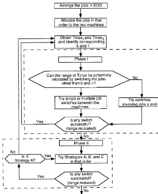
Consider an allocation of the jobs to the two machines with the jobs assigned to the machines in the EDD order, as described above. First consider the single job exchange. Let Job i from Machine 1 be exchanged with Job j from Machine 2 such that i.b.j, and i and j are not the jobs with the
¹
.!91and¹.!92values, respectively. Letpiandpjbe
their respective processing times. Such an exchange is shown in Fig. 4.
Theorem 1. Under single job exchange, both
¹
.!91and¹.!92decrease simultaneously if and only if there exist a Job i on Machine 1 and a Jobj on Machine 2 such that
p
i(pj and di)dk(dj)dl,
where k and l are the jobs corresponding to the
¹
.!91and¹.!92values, respectively.
Proofs of Theorem 1, and Theorems 2 and 4 to follow, are given in the Appendix.
Next, we precisely develop the conditions for the exchange of Jobsiandjto result in the¹
.!9value less than min(¹
.!91,¹.!92). Such an exchange of
Jobsi andjwill be called a successful exchange.
Theorem 2.
(a) If ¹
k'¹l, the conditions for a successful ex-change are:
(i) there exists a Jobion Machine 1 such that
p
i¹k!¹l#1 and d
i*dk (if more than
one Jobiexist then we select a job with the minimum processing time and designate it byp
i.*/);
(ii) there exists a Jobjon Machine 2 such that
d
k(dj)dlandp
j'pi.*/;
(iii) for Jobs q on Machine 2 such that
d
i)dq)dj,¸q)¹l!(p
i.*/#1); (iv) for Jobs m on Machine 1 such that
d
m*dj,¸m)¹l!(p
j!pi.*/)!1;and (v) the tardinesses of the Jobsiandj, after the
move, are less than¹l (b) If ¹
k)¹l, the necessary conditions for a suc-cessful exchange are:
(i) there exists a Jobion Machine 1 such that
d
i(dk(if more than one Jobiexist, then we
select min suchiand designate it byp
(ii) for any Job m on Machine 1 such that
d
m'dj,¸m)(¹k!¹l)#¹ k!2; (iii) for any Job q on Machine 2 such that
d
i)dq)dj,¸q)¹k!(pi.*/#1); and (iv) the tardinesses of the Jobsiandj, after the
move, are less than¹
k.
The conditions in Theorem 2 indicate that if any one of them is violated, then it is not possible to get
a schedule with the ¹
.!9 value less than min(¹
k,¹l). Note that condition (iii) of Theorem 2(b) can be relaxed for implementation purposes by considering Job q s.t. d
i)dq)ds (instead of
d
i)dq)dj), where ds)dj for all Jobs j on Machine 2 s.t.d
k(dj(dl.
4.1.1.1. Extension to multiple job exchange. The above discussion was focused on the exchange of a single Jobion Machine 1 with a single Jobjon Machine 2. However, the arguments presented can easily be extended to the exchange of multiple jobs. Conditions for this case are equivalent to those in Theorem 2 and can be developed to be the following.
Case (a):¹
k'¹l
(i) there exists a set of Jobs A on Machine 1 (equivalent of Jobibefore) such thatd
a)dk for alla3Aand+a|Ap
a*¹k!¹l#1. (ii) there exists a set of Jobs B on Machine
2 (equivalent of Job j before) such that
d
k(d)dlfor all b3Band +
b|Bpb'+a|Apa. (Note that the setsAorBcould be singletons.) (iii) Ifj
1represents a job amongst the jobs inBwith the minimum due date, then for all q)Qon Machine 2 s.t. d
i(dq(dj(where Job iis the single job being exchanged with a set of Jobs
B),¸
q3¹l!(+
a|Apa#1). (iv) If j
2 represents the job with the highest due date among those in the set B, then
¸
In case multiple jobs can be found that meet condition (i), determine a set of jobs to be switched by solving the knapsack problem: +
a{pa{xa{ s.t. +
a{pa{xa{*v; wherev"¹k!¹l#1 to start with.
If there is an alternative optimum, then select a solution for which the last a@job, with xa@"1, has maximum da@. Call this job llast. If
¸
Multiple jobs for switching are determined by generating combinations of the jobs that satisfy the speci"ed condition to belong in Set A. Various combinations of the jobs of increasing cardinality are generated systematically. Whenever, a combi-nation of the jobs is found (with respect to SetA), then the best combination of the jobs of that car-dinality is selected to switch. Thus, the knapsack problem is solved heuristically using partial enu-meration.
Case (b):¹
k)¹l
(i) there exists a set of JobsAon Machine 1 and a set of Jobs B on Machine 2 such that (ii) for all Jobs m on Machine 1 such that
d
m'dl,¸
m)(¹k!¹l)#(¹ k!2).
(iii) ifdis the highest due date job among the jobs aandbde"ned in (i), andorepresents the job with the highest due date among those in B
2
(iv) the tardinesses of the jobs in SetsAandB, after the move, are less than¹
k.
4.1.2. Analysis for the case when the jobskandlare
exchanged
Now, consider the case when the jobs considered for exchange, namely, Job i or Job j (or both) correspond to the Jobskandl. This can lead to the consideration of the following three di!erent cases.
Case 1: Job k is moved from Machine 1 to Machine 2 but Joblis not.
Case 2: Job l is moved from Machine 2 to Machine 1 but Jobkis not.
Consider Case 1. As in either of the two situations, value, we require that
a. Some Job&m'such thatm.b.kshould be shifted from Machine 2 to Machine 1.
b. If Jobkis the"rst of the jobs in the sequence to be shifted from one machine to another, then it should be moved such that it gets an earlier start time on Machine 2. Also, we would require thatp
m(pkbecause, otherwise for some Job&q' on Machine 1 such that q.b.k, its completion time value obtained after the exchange would be greater than the completion time value of Job k before the exchange thus leading to a higher tardiness value.
c. If Jobkis moved from Machine 1 to Machine 2 and Jobmfrom Machine 2 to Machine 1 with
m.b.kandp
m(pkthen it is necessary to move Job l from Machine 2 to Machine 1 because otherwise there would be an increase in the completion time of Joblon Machine 2 and this is not desired. Thus, we note that Case 1 be-comes identical with Case 3.
As regards Case 2, it is necessary to move some Job iwith i.b.kfrom Machine 1 to Machine 2 so that the tardiness value of Job kdecreases. Now, considering the situations pertaining to (a)¹
k(¹l and (b)¹
k*¹l, the analysis becomes identical to that of the analysis presented in Section 4.1.1 (when the jobs with¹
.!9values are not exchanged) with only Job j being replaced by Jobl. Hence, we note that in this context the only case that demands further discussion is Case 3, that is, when both Job
kand Joblare shifted. In this case, as described above in Case 1, we would shift Job msuch that
m.b.k from Machine 2 to Machine 1, Job k
from Machine 1 to Machine 2 and Job l
from Machine 2 to Machine 1. Extension of this argument to the case of multiple job exchange would require the interchange of Jobkand a set of Jobs A from Machine 1 for which d
a(dk for all a3A, with a set of JobsBfrom Machine 2 for which
d
b(dkfor all b)B, such that+bpb!+apa(pk and Jobl.
Note that Theorem 1 speci"es both the necessary and su$cient conditions for the relocation of
¹H
.!9range. Conditions of Theorem 2 and the sub-sequent development for multiple job exchange and the exchange of¹
.!9jobs are all based on the result of Theorem 1 and hence lead to the conclusion of the following result.
Theorem 3. If for a given allocation of the jobs to the two machines with¹M
.!9"min(¹.!91,¹.!92), single and multiple job exchangesviolate the conditions of Theorem 2 (and subsequent ones for multiple jobs) and those for the case when the¹
.!9jobs on both the
machines are also exchanged, then¹H
.!9*¹M .!9. Moreover, it is clear that¹H
.!9)max(¹.!91,¹.!92).
Hence, the Phase I analysis results in an upper and lower bound on¹H
.!9.
4.2. Analysis to constrict the range obtained
(Phase II)
Now that (as a result of Phase I) we have an assignment of the jobs on the two machines such that no change in the assignment would lead to a value of¹
.!9 less than min(¹k,¹l), we reassign the jobs so as to constrict the range over which the
¹
.!9 value lies. The aim is to constrict it to an extent that either it becomes small enough to satisfy a prespeci"ed value or it cannot be reduced any more.
Constriction of range is done by following strat-egies, A,B or C (described earlier in Section 3) depending upon the locations of the jobs from Machines 1 and 2 that are considered for exchange. If the exchange procedure uses StrategyAthen it is obvious that we have a new set of values¹
kand
¹l such that the optimal value of ¹
.!9[¹k,¹l] because it reduces the maximum of the two
¹
.!9values. In case of the use of StrategiesBorC, as the minimum of¹
.!91 and¹.!92 increases, it is
necessary to verify once again if the optimal value of ¹
.!9 lies over the new range corresponding to the new¹
kand¹lvalues obtained. This is checked by applying Phase I. This results in the identi" ca-tion of a range smaller than before over which the optimal ¹
The analysis is divided into two cases depending
Strategy A: To implement this strategy, select a Jobjfrom Machine 2 such thatd
k(dj)dl(so that¹
kis not a!ected), and that for all JobsQon Machine 1 withd
j(dq,q3Q,¸q#pj)¹lso that the tardiness of any job does not exceed¹l. Also, in order that the value of¹ldoes not decrease beyond the value of ¹
k, the processing time of the Job
j transferred from Machine 2 to Machine 1 with
d
k(dj)dl, and j.b.l, should be such that ¹l!p
j*¹k or ¹l!¹
k*pj. A more general way of following Strategy A is by the exchange of multiple Jobs i on Machine 1 with multiple Jobs &j' on Machine 2 such that +p
i(+pj and
¹l!¹
k*+pj!+pi.
Strategy B:For a job exchange that follows this strategy, we would consider the transfer of a single Job j from Machine 2 to Machine 1 such that
d
j(dk(designated as exchange of Type 1), or the exchange of a Jobifrom Machine 1 with Jobjfrom Machine 2 such that p
j'pi,di)dk and dj(dk (designated as exchange of Type 2)
Since we are interested in having the"nal values of ¹
k and¹l(i.e. the values after the exchange of jobs) to lie in the closed interval [¹
k,¹l], in the exchange of Type 1 we require that¹
k#pj(¹lor The tardiness values of the appropriate sets of jobs on Machines 1 and 2 should not violate this condi-tion as well. For instance, ifi.b.j,¸
m#pi)¹l!1 for i.b.m.b.j, and if j.b.i,¸
m#pj)¹l!1 for
j.b.m.b.l.
The exchange of Type 2 can be generalized to the exchange of multiple Jobs ifrom Machine 1 with multiple Jobs j from Machine 2 such that
+p
j!+pi(¹l!¹
kwith the tardiness values of the appropriate sets of jobs on Machines 1 and 2 not violating this condition.
Strategy C:To implement this strategy, exchange Job i from Machine 1 with Job j from Machine 2 such thatp
i"pj,dj(dkanddk(di(dl. Case b:¹
k'¹l
Strategy A: In this case, exchange Job i from Machine 1 with Job j from Machine 2 such that
p
i"pj,di(dkanddk(dj(dl, with the tardiness
value of none of the jobs on Machine 2 in between Jobsi andjto exceed¹l.
Strategy B:This would require either the transfer of a single Jobifrom Machine 1 to Machine 2 such thatd
i(dk(exchange of Type 1) or the exchange of Job i from Machine 1 with Job j from Machine 2 such thatp
i'pj,di(dkanddj)dk(exchange of Type 2). The restriction of the"nal values of¹
kand
¹l to the closed interval [¹l,¹
k] would require thatp
i)¹k!¹l in case of exchange of Type 1, and p
i!pj)¹k!¹l in case of exchange of Type 2 with the tardiness values of the appropriate sets of jobs on Machines 1 and 2 not violating this condition as well.
Strategy C:This would require either the transfer of a single Jobifrom Machine 1 to Machine 2 such thatd
k)di)dlor the exchange of Jobion Ma-chine 1 with Job j on Machine 2 such that
p
i'pj,dk(di(dlandd
k(dj(dl. Moreover, to restrict the"nal values of¹
kand¹lto the closed interval [¹l,¹
k] requires restrictions on pi and
p
i!pjas mentioned above in Strategy B.
4.3. Optimality of the procedure
Theorem 4. Repeated Application of Phase I and
Phase II will result in the attainment of¹H
.!9. This result indicates to stop performing job switches between the machines when both Phase I and Phase II exchanges are not successful.
5. Algorithm to minimize¹
.!9
Next, we present the ¹
.!9 minimization algo-rithm. It incorporates only selected job exchanges, namely those involving single jobs and contiguous jobs. As a result, it does not guarantee attainment of the optimal solution. However, the algorithm is e$cient and the experimentation, reported later, indicates that it generates almost optimal solutions. An outline of the algorithm is given in Fig. 5.
Step 1:
Arrange all the jobs in the EDD order and if
d
Fig. 5. An outline of the¹
.!9Algorithm.
Step 2:
Allocate the jobs in that order on the two ma-chines such that each job gets the earliest pos-sible start.
Step 3:
Designate¹
.!91 and ¹.!92 by ¹k and ¹l such
that k.b.l with the machine to which Job k belongs denoted as Machine 1 and the other machine denoted as Machine 2.
Phase I (Range Relocation Phase)
Step 4:
Does there exist a Jobjon Machine 2 such that
k.b.j.b.l
if no, then go to Step 7 else go the Step 5.
Step 5: (Execute this step to relocate the range if
¹
k'¹l) if¹
k'¹lthen
try single and multiple job switches between the machines for successful range relocation by checking the necessary conditions (i) to (v) of Theorem 2(a).
if max(¹
if no single or multiple Job j can be found that satisfy conditions of Theorem 2(a), then go to Step 7. else continue
else max(¹
knew,¹lnew)(¹l, switch is successful in relocating range and exit to Step 3.
else go to Step 6.
Step 6:(Execute this step to relocate the range when
¹
k)¹l)
if k"1, then no Job i can be found, so go to Step 7.
else determine a single or multiple Job i to be switched with a single or multiple Job j that satisfy all conditions of Theorem 2(b).
if max(¹
knew,¹lnew)(¹
k, then go to Step 3
else determine new sets of jobs to be switched if no jobs can be found for switching, then go to Step 7
else, continue to"nd new sets of jobs.
Step 7:(Execute this job to exchange Jobskandl). This is done in accordance with the earlier dis-cussion in Section 4.1.2. We do not consider here exchanges of multiple jobs between the machines for the sake of simplicity.
Set¸B
m"0
if there exists a jobmon Machine 2 such that
¸B
m.b.m.b.kandpm(pk then select m such that p
m is minimum; shift Jobmto Machine 1, Jobkto Machine 2, and Job l to Machine 1.
if max(¹
knew, ¹l new)(max(¹ k,¹l), then go to Step 3
else put the jobs to their original posi-tions, set¸B
m"m and try to"nd an-otherm.
else range cannot be relocated, go to Step 8. Phase II (Range Reduction Phase)
Step 8:(Phase II for the case when¹
k)¹l.) Once a range is established over which the
¹
.!9 value lies, an attempt is made to reduce it by using the strategies described in Section 4.2.
if¹
k'¹l, then go to Step 9
else try Strategy A, then B and then C as described in Case (a) of Section 4.2.
In Strategy B, "rst try exchange Type 1 and then exchange of Type 2.
if a switch is successful, then
if it is successful due to Strategies
BorC, then exit to Step 3
else try StrategiesA,B, andCagain else go to Step 10.
Step 9:(Phase II for the case when¹
k'¹l) First, try StrategyAfollowed by the exchange of Type 1 and then of Type 2 under StrategyBas described in Case (b) of Section 4.6 and imple-mented in Step 8 except that now the roles of Machine 1 and Machine 2 are switched, and then try StrategyCin that order.
if a switch is successful, then
if it is successful due to StrategiesBand/or
C, then exit to Step 3
else try StrategiesA,B, andCagain. else go to Step 10.
Step 10:
Determine¹
kand¹lfor the current schedule. The best value of¹
.!9obtained"max(¹k,¹l).
6. Minimization of the secondary criterion
As alluded to earlier, a branch and bound based method is used to min NT given the¹
.!9value. It proceeds by scheduling the jobs backwards on both the machines. To implement it, we"rst need to"x the makespan on both the machines and then make the job allocations. IfC
1andC2are the makespan values on Machines 1 and 2, thenC#C
2is equal to the sum of the processing times of the jobs, and is constant. Therefore, for a given C
1 there corres-ponds a de"nite value ofC
2. If d
.!9 denotes the maximum among the due date values, then the maximum possible value of
C
1 that does not violate the primary criterion is
d primary criterion. That is, if the jobs are scheduled backwards starting from a set ofC
NT and¹
.!9criteria. The schedules with gaps will be referred to as infeasible schedules. However, we know that there does exist at least one feasible set of
C
1 and C2 values (in particular, the makespan values corresponding to the schedule that opti-mizes the primary criterion) that gives a feasible set of makespan values.
In the algorithm presented, we begin by examin-ing various possible assignments beginnexamin-ing with a makespan value C
1"d.!9#¹H.!9 on Machine 1 and the corresponding value ofC
2on Machine 2. If a certain value ofC
1is found to be infeasible, we proceed to the next possible value ofC
1. The pro-cedure is continued until all possible values of
C
1are covered.
6.1. Algorithm to minimize the number of tardy jobs
LetN¹
i"the number of tardy jobs obtained so far in any branchi;;B"the upper bound value
on the number of tardy jobs; and ¹
.*/641(i) and
¹
.*/642(i) be the values of time on the two machines for active branchi.
Step 1: Initialization.
Let C
1"d.!9#, and de"ne C2 accordingly. Without loss of generality, letC
1*C2(that is, the machine with the larger makespan is desig-nated as Machine 1). Let UB"the number of tardy jobs in the schedule obtained for the
¹
Determine the set of jobs (designated eligible jobs) which have not been scheduled so far and which when scheduled to end at TimeFwould not have a tardiness value greater than ¹H
.!9. Note that this would also include the jobs that would be early if scheduled to end at that posi-tion. If no job is eligible, fathom that branch and go to Step 5.
Step 4:
For each eligible Jobi, branch out by scheduling Job i to end at Time F on the machine from which the value of F was obtained. Determine the corresponding starting TimeS
1orS2of the job on Machine 1 or 2 wherever scheduled. If for any branch S
1(0 or S2(0, fathom that
branch (implying an infeasible assignment as the job starting time precedes machine availability time). Also, fathom a branch if max(S
1,S2)"0. This indicates the attainment of a feasible sched-ule. If F)d
i, then set the NT value for this branch equal to the NT value of the parent
branch. Otherwise, NT value of this
branch"NT value for the parent branch#1 (if NT*UB, then fathom this node). Store the values ofS
1andS2for each branch in the arrays named¹
.*/641and¹.*/642. If there are two jobs with the same processing time eligible to be scheduled at a position, store the schedule corre-sponding to the job that would not be tardy at that position, otherwise store the schedule corre-sponding to any one of them. Determine the NT value of a branch with the max(S
1,S2)"0, and set UB"min (UB, NT).
Step 5:
Set S"max
ixANMmax[¹.*/641(i),¹.*/642(i)]N, where AN refers to the set of activenodes. If AN"/, then go to Step 6. Letkbe the value of
i corresponding to S. Set S
1"¹.*/641(k)
The current value of the upper bound (UB) gives the optimal value of NT. Stop.
6.2. Determination of lower and upper bounds for number of tardy jobs
Tighter upper and lower bound values can be computed as follows. These are however not imple-mented in the above algorithm. A tighter lower bound value for each node can be obtained by scheduling the remaining jobs (jobs not scheduled so far) on a single machine and minimizing the number of tardy jobs in this set, for a given value of
¹
Table 1
Average execution time vs. problem size for the¹
.!9 minimiz-ation algorithm
Problem number
Problem size (n)
Average execution time of ten observations (s)
1 50 0.13
2 100 0.34
3 150 0.70
4 200 1.20
5 250 1.86
6 300 2.61
7 350 3.65
8 400 4.57
9 450 5.75
10 500 7.08
¹
.!9 for the single machine problem can be ob-tained from the EDD sequence. A tighter upper bound can be obtained by minimizing the number of tardy jobs on each machine individually by using the single machine algorithm [8,9] for the assign-ment of jobs obtained as a result of the¹
.!9 prob-lem. This involves the solution of two single machine problems.
7. Experimental results
The algorithms suggested above were coded in FORTRAN-77 and were run on an IBM 3090.
7.1. ¹
.!9minimization algorithm For the algorithm to minimize ¹
.!9, problems were generated using the due date procedure sim-ilar to the one suggested by Emmons [10]. In this procedure, the processing times are selected as uni-formly distributed integer values between 1 and
u(whereuis an integer). Problems were generated for various values ofu. The due date for each job is determined by adding a number randomly selected from a uniform distribution of integers between 0 andn, where&n'represents the number of jobs:
d
i"pi#;(0,n).
The results obtained regarding the variation of average execution time vs. the problem size are presented in Table 1. Ten problems were run for each problem size. Note that if for a solution, D¹
k!¹lD is at most 1 and no j exists such that
k)j)l, then many of the exchanges need not be tested. Also, if other exchanges are not successful, then that is an optimal solution. This criterion was satis"ed in all the problems that were run.
As mentioned earlier, the jobs are initially as-signed to the machines in EDD order with each job assigned to the earliest available machine. This initial assignment tends to minimize the number of jobs between Jobskandl, and consequently makes the algorithm an e!ective one, on the average. Also, in the experimentation, it is observed that with this starting solution Phase I exchanges are successful only occasionally. However, if the jobs are initially assigned to machines di!erently, quite a few
suc-cessful exchanges are carried out in Phase I of the algorithm, and consequently, the computational time also increases.
To further study the behavior of the algorithm, problems were run for di!erent values ofu, and for di!erent types of due dates and processing times. Table 2 shows the variation of the number of iter-ations required to solve the problem with di!erent values of u (for a constant value of n"1000). As Phase I exchanges were successful only occa-sionally, each iteration here refers to the successful execution of the range reduction step (Phase II). So, in other words, the number of iterations also indi-cate the number of times range reduction is ac-complished. We observe that the number of iterations required to solve the problem increases withu(i.e. the greater the variation in job process-ing times, the greater is the number of iterations required in the knapsacks involving p
i!pj). As regards di!erent values of the due dates and pro-cessing times, the type of problem that showed the worst kind of computational complexity has rela-tively small processing times for most of the jobs in between Jobskandl, and the due dates for these jobs are such that they do not become too tardy while the processing times of both the Jobskand lare very large thereby delaying them by a large amount.
Table 2
Average number of iterations vs. range of processor times for the ¹
.!9minimization algorithm Range of processing times (1,u)
Average no. of iterations of ten observations for problems for sizen"1000
(1, 10) 2
(1, 250) 7
(1, 100) 11
(1, 200) 13
(1, 300) 17
(1, 500) 30
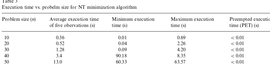
Table 3
Execution time vs. probelm size for NT minimization algorithm Problem size (n) Average execution time
of"ve obervations (s)
Minimum execution time (s)
Maximum execution time (s)
Preempted execution time (PET) (s)
10 0.36 0.01 0.69 (0.01
20 0.52 0.04 2.26 (0.01
30 1.28 0.09 4.20 (0.01
40 3.4 90.18 8.35 (0.01
50 13.0 60.33 63.57 (0.01
75 '600 0.56 '600 0.85
100 '600 '600 '600 2.81
starting with the EDD sequence, the computational experience indicates attainment of fairly good solu-tions.
7.2. NT minimization algorithm
Computational experience with this algorithm indicates that the high storage requirements for this algorithm restrict its application to problems of size
n)100. To study the behavior of the algorithm for the problems generated, the processing times were chosen such thatp
i";(1, 10). The due dates were chosen in the same manner as that for the problem to minimize the value of¹
.!9. A lower bound value was calculated for each node as described earlier. The nodes with lower bound values greater than the current upper bound are fathomed.
Table 3 shows the variation of execution time vs. problem size. The observations presented in the table are based on the results for "ve di!erent problems of each size. Columns 2}4 report the
average CPU time and the range of CPU time in seconds required to obtain the optimal solutions. Also, we show CPU time required to reach a stage when the least lower bound on the number of tardy jobs does not di!er from the upper bound value by more than 1. This is called &preempted execution time'and is designated by PET, also depicted in the last column of Table 3. Note that PET is relatively very small for the problems tested (negligible for problems of size up ton"50), while the CPU time to obtain an optimal solution took more than 600 s for all the problems of sizen"100 and for some problems of sizen"75.
As a"nal note, the upper bound value computed based on solution to two single machine problems (as described in Section 6.2) was found to be quite close to the optimal solution. Hence, as an approx-imate solution, one can apply single machine NT algorithm to the job allocations on the machines obtained as a result of¹
.!9algorithm. Problems of size up to 1000 jobs can be easily solved by this procedure.
8. Concluding remarks
In this paper, we have developed algorithms for a bicriteria problem involving the minimization of
¹
.!9as the primary criterion and the minimization of NT as the secondary criterion. Both the algo-rithms are quite e!ective to use. The¹
problems of size up to 100 jobs beyond which it encounters storage problems. An approximation to this procedure is also suggested which tremendous-ly cuts down the computational time; and due to another approximation even problems of up to 1000 jobs can be easily solved.
Future work in the two machine bicriteria prob-lem can be devoted to other pairs of criteria involv-ing NT and¹
.!9, total completion time and¹.!9, total tardiness and¹
.!9, and NT and total comple-tion time as primary and secondary criteria. Also, a natural extension of this work would be to con-sider probabilistic processing times instead of de-terministic values considered here.
Acknowledgements
The authors are thankful to the reviewers and Dr. Salah Elmaghraby of North Carolina State Univer-sity for providing several insightful suggestions that helped improve the quality of presentation.
Appendix A
Proof of Theorem 1.Sincei.b.k,¹
.!91decreases by
p
crease or remain the same.
Proof of Theorem 2. (a) Sinced
i)dk(dj(by The-Considering the processing times and due dates of the jobs to be integer values, we require that
p tion times and latenesses of these jobs, respectively, before and after the exchange of Jobs i and j. Clearly C@
q,"Cq#pi.*/, and ¸@q"¸q#pi.*/. In
order to obtain a successful exchange, we require that ¸@
Now, for any Job m on Machine 1 such that
d
m*dj the completion time after the exchange increases by a value of p
j!pi.*/ with pj'pi.*/ (by Theorem 1). Hence, C@
m"Cm#(pj!pi.*/) which further implies that ¸@
m¸m#(pj!pi.*/). Since for a successful exchange we require that
¸@
k#1 (again by assuming that allpand¹values are integers). For any Jobmon Machine 1 such thatd
m*dj, the value of lateness after exchange is ¸@
m"¸m#(pj!pi.*/). In ac-cordance with the above requirement, we have,
¸
k#2. As the latest possible position of Jobjcan bel, the necessary condition is that ¸
m)(¹k!2)!(¹l!¹
k) for all Jobs m on Machine 1 such thatd
m*dl.
Next, consider any Jobqon Machine 2 such that
d
i)dq)dj. The lateness value ¸@q after the ex-change would be ¸@
q"¸q#pi.*/. Again, we re-quire that ¸@
q(¹k, which after substituting for
¸@
qbecomes ¸q#pimin(¹k, Thereby leading to the necessary condition of¸
q)¹k!(pi.*/#1).
Proof of Theorem 4. Single and multiple job
ex-changes are performed in accordance with the con-dition of exchange that are derived from the result of Theorem 1. Repeated application of Phase I and Phase II results in the monotone reduction of the range over which¹H
.!9lies. Eventually, this range becomes zero or no more exchange is possible which can further decrease this range, thereby resulting in the optimal solution.
References
[2] A.A. Cenna, M.T. Tabucanon, Bicriterion scheduling prob-lem in a job shop with parallel processors, International Journal of Production Economics 25 (1}3) (1991) 95}101. [3] R.L. Daniels, R.J. Chambers, Multiobjective #ow-shop
scheduling, Naval Research Logistics 37 (1990) 981}995. [4] M.R. Garey, D.S. Johnson, Two processor scheduling with
start-times and deadlines, SIAM Journal on Computer 6 (3) (1977) 416}426.
[5] W. Townsend, Sequencingnjobs onmmachines to minim-ize maximum tardiness: A branch and bound procedure, Management Science 23 (9) (1977) 1016}1019.
[6] T.S. Nunnikhoven, H. Emmons, Scheduling on parallel machines to minimize two criteria related to job tardiness, AIIE Transactions 9(3) (1977) 288}296.
[7] A.H.G. Rinnooy Kan, Machine Scheduling Problems: Classi"cation, Complexity and Computations, Martinus Nijho!, The Hague, 1976.
[8] R.T. Nelson, R.K. Sarin, R.L. Daniels, Scheduling with multiple performance measures: The one ma-chine case, Management Science 32 (4) (1986) 464}480.
[9] S.C. Sarin, R. Hariharan, Single Machine Bicriteria Sched-uling Problem, Virginia Polytechnic Institute and State University, Blacksburg, VA, 24061.