www.elsevier.com/locate/spa
A partial introduction to nancial asset pricing theory
(Philip Protter
a;b;∗aOperations Research and Industrial Engineering Department, Cornell University, Ithaca, NY 14853, USA
bMathematics and Statistics Departments, Purdue University, W. Lafayette, IN 47907-1395, USA
Received 11 March 2000; received in revised form 16 June 2000; accepted 19 June 2000
Abstract
We present an introduction to mathematical Finance Theory for mathematicians. The approach is to start with an abstract setting and then introduce hypotheses as needed to develop the theory. We present the basics of European call and put options, and we show the connection between American put options and backwards stochastic dierential equations. c 2001 Elsevier Science B.V. All rights reserved.
Keywords:Financial asset pricing theory; Options; Arbitrage; Complete markets; Numeraire invariance; Semimartingale; Backwards stochastic dierential equations
1. Introduction
Stock markets date back to at least 1531, when one was started in Antwerp, Belgium. Today there are over 150 stock exchanges (see Wall Street Journal, May 15, 2000). The mathematical modeling of such markets however, came hundreds of years after Antwerp, and it was embroiled in controversy at its beginnings. The rst attempt known to the author to model the stock market using probability is due to L. Bachelier in Paris about 1900. Bachelier’s model was his thesis, and it met with disfavor in the Paris mathematics community, mostly because the topic was not thought worthy of study. Nevertheless we now realize that Bachelier essentially modeled Brownian motion ve years before the 1905 paper of Einstein (albeit twenty years after T. N. Thiele of Copenhagen (Hald, 1981)) and of course decades before Kolmogorov gave mathematical legitimacy to the subject of probability theory. Poincare was hostile to Bachelier’s thesis, remarking that his thesis topic was “somewhat remote from those our candidates are in the habit of treating” and Bachelier ended up spending his career in Besancon, far from the French capital. His work was then ignored and forgotten for some time.
(Supported in part by NSF grants # 9971720-DMS and 9401109-INT, and NSA grant #
MDA904-00-1-0035.
∗Correspondence address: Operations Research and Industrial Engineering Department, Cornell University,
Ithaca, NY 14853, USA.
Following work by Cowles (1930s), Kendall and Osborne (1950s), it was the re-knowned statistician L. J. Savage who re-discovered Bachelier’s work in the 1950s, and he alerted Paul Samuelson (see Bernstein, 1992, pp. 22–23). Samuelson further developed Bachelier’s model to include stock prices that evolved according to a geo-metric Brownian motion, and thus (for example) always remained positive. This built on the earlier observations of Cowles and others that it was the increments of the logarithms of the prices that behaved independently.
The development of nancial asset pricing theory over the 35 yr since Samuelson’s (1965) article has been intertwined with the development of the theory of stochastic integration. A key breakthrough occurred in the early 1970s when Black and Scholes (1973) and Merton (1973) proposed a method to price European options via an explicit formula. In doing this they made use of the Itˆo stochastic calculus and the Markov property of diusions in key ways. The work of Black et al. brought order to a rather chaotic situation, where the previous pricing of options had been done by intuition about ill-dened market forces. Shortly after the work of Black et al. the theory of stochastic integration for semimartingales (and not just Itˆo processes) was developed in the 1970s and 1980s, mostly in France, due in large part to P. A. Meyer of Stras-bourg and his collaborators. These advances in the theory of stochastic integration were combined with the work of Black et al. to further advance the theory, by Harrison and Kreps (1979) and Harrison and Pliska (1981) in seminal articles published in 1979 and 1980. In particular they established a connection between complete markets and martingale representation. Much has happened in the intervening two decades, and the subject has attracted the interest and curiosity of a large number of mathematicians. The interweaving of nance and stochastic integration continues today. This article has the hope of introducing mathematicians to the subject at more or less its current state, for the special topics addressed here. We take an abstract approach, attempting to in-troduce simplifying hypotheses as needed, and we signal when we do so. In this way it is hoped that the reader can see the underlying mathematical structure of the theory. The subject is much larger than the topics of this article, and there are several books that treat the subject in some detail (e.g., Due, 1996; Karatzas and Shreve, 1998; Musiela and Rutkowski, 1997; Shiryaev, 1999). Indeed, the reader is sometimes referred to books such as (Due, 1996) to nd more details for certain topics. Otherwise references are provided for the relevant papers.
2. Introduction to options and arbitrage
Let X = (Xt)06t6T represent the price process of a risky asset (e.g., the price of a
stock, a commodity such as “pork bellies,” a currency exchange rate, etc.). The present is often thought of as time t= 0; one is interested in the price at time T in the future which is unknown, and thus XT constitutes a “risk”. (For example, if an American
The payo at time T of a call option with strike priceK can be represented math-ematically as
H(!) = (XT(!)−K)+;
where x+= max(x;0). Analogously the payo of a put option with strike price K at
time T is
H(!) = (K−XT(!))+;
and this corresponds to the right to sell the security at price K at time T.
These are two simple examples, often called European call options and European put options. They are clearly related, and we have
XT−K= (XT−K)+−(K−XT)+:
This simple equality leads to relationships between the price of a call option and the price of a put option, known as put–call parity. We return to this in Section 3.7. We can also use these two simple options as building blocks for more complicated ones. For example if
H= max(K; XT)
then
H=XT+ (K−XT)+=K+ (XT −K)+:
More generally if f: R+→R+ is convex we can use the well known representation
f(x) =f(0) +f′+(0)x+ Z ∞
0
(x−y)+(dy) (1)
wheref+′(x) is the right continuous version of the derivative off, and is a positive measure on R with=f′′, where the derivative is in the generalized function sense.
In this case if
H=f(XT)
is our contingent claim, thenH is eectively a portfolio of European call options, using (1) (see Brown and Ross, 1991):
H=f(0) +f+′(0)XT+
Z ∞
0
(XT−K)+(dK):
For the options discussed so far, the contingent claim is a random variable of the form H=f(XT), that is, a function of the value ofX at one xed and prescribed time
T. One can also consider options of the form
H=F(X)T
=F(Xs; 06s6T)
which are functionals of the paths ofX. For example if X has cadlag paths (cadlag is a French acronym for “right continuous with left limits”) thenF:D→R+, whereDis the space of functionsx: [0; T]→R+ which are right continuous with left limits. If the
be European options, although their analysis for pricing and hedging is more dicult than for simple call and put options. AnAmerican optionis one which can be exercised at any time before or at the expiration time. That is, an American call option allows the holder to buy the security at a striking price K not only at timeT (as is the case for a European call option), but at any time between times t= 0 and time T. (It is this type of option that is listed, for example, in the “Listed Options Quotations” in the Wall Street Journal.) Deciding when to exercise such an option is complicated. A strategy for exercising an American option can be represented mathematically by a
stopping rule . (That is, if (Ft)t¿0 is the underlying ltration of X then {6t} ∈Ft
for each t; 06t6T.) For a given , the claim is then (for a classic American call) a payo at time (!) of
H(!) = (X(!)(!)−K)+:
We now turn to the pricing of options. Let H be a random variable in FT
rep-resenting a contingent claim. Let Vt be its value (or price) at time t. What then
is V0?
From a traditional point of view, classical probability tells us that
V0=E{H}: (2)
One could discount for the time value of money (ination) and assuming a xed interest rate r and a payo at time T, one would have
V0=E
H
(1 +r)T
(3)
instead of (2). For simplicity we will take r= 0 and then show why the obvious price given in (2) does not work (!). For simplicity we consider a binary example. At time
t= 0; 1 Euro = $1:15. We assume at time t=T the Euro will be worth either $0:75 or $1:45; the probability it goes up to $1:45 is p and the probability it goes down is 1−p.
Let the option have exercise price K=$1.15, for a European call. That is, H= (XT −
$1:15)+, where X = (X
rules for calculating probabilities dating back to Huygens and Bernoulli give a price of H as
E{H}= (1:45−1:15)p= (0:30)p:
For example if p= 1=2 we get V0= 0:15.
TheBlack–Scholesmethod1 to calculate the option price, however, is quite dierent.
We rst replace p with a new probability p∗ that (in the absence of interest rates) makes the security price X = (Xt)t=0; T a martingale. Since this is a two-step process,
we need only to choose p∗ so that X has constant expectation. Since X0= 1:15, we
need
E∗{XT}= 1:45p∗+ (1−p∗)0:75 = 1:15;
whereE∗ denotes mathematical expectation with respect to the probability measure P∗
given by P∗(Euro = $1:45 at time T) =p∗, and P∗(Euro = $0:75 at timeT) = 1−p∗. Solving for p∗ gives
p∗= 4=7:
We get now
V0=E∗{H}= (0:30)p∗= 6=35≃0:17: (4)
The change from p to p∗ seems arbitrary. But there is an economics argument to justify it; this is where the economics concept of theabsence of arbitrage opportunities
changes the usual intuition dating back to the 16th and 17th centuries.
Suppose, for example, at time t= 0 you sell the option, giving the buyer of the option the right to purchase 1 Euro at time T for $1:15. He then gives you the price
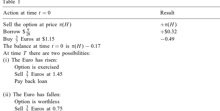
(H) of the option. Again we assume r= 0, so there is no cost to borrow money. You can then follow a safety strategy to prepare for the contingent claim you sold (see Table 1, calculations are to two decimal places):
Since the balance at time T is zero in both cases, the balance at time 0 should also be 0; therefore we must have (H) = 0:17. Indeed any price other than (H) = 0:17 would allow either the option seller or buyer to make a sure prot without any risk: this is called an arbitrage opportunity in economics, and it is a standard assumption that such opportunities do not exist. (Of course if they were to exist, market forces would, in theory, quickly eliminate them.)
Thus we see that — at least in the case of this simple example — that the “no arbitrage price” of the contingent claim H is not E{H}, but rather must be E∗{H},
since otherwise there would be an opportunity to make a prot without taking any risk. We emphasize that this is contrary to our standard intuition, since P is the probability measure governing the true laws of chance of the security, while P∗ is an articial construct.
Table 1
Action at timet= 0 Result
Sell the option at price(H) +(H)
Borrow $289 +$0:32
Buy 3
7 Euros at $1:15 −0:49
The balance at timet= 0 is(H)−0:17 At timeT there are two possibilities: (i) The Euro has risen:
Option is exercised −0:30
Sell 37 Euros at 1.45 +0:62
Pay back loan −0:32
0 (ii) The Euro has fallen:
Option is worthless 0
Sell 37 Euros at 0.75 +0:32
Pay back loan −0:32
0
This simple binary example can do more than illustrate the idea of using lack of arbitrage to determine a price. We can also use it to approximate some continuous models. We let the time interval become small (t), and we let the binomial model already described become a recombinant tree, which moves up or down to a neighboring node at each time “tick” t. For an actual time “tick” of interest of length say , we can have the price go to 2n possible values for a given n, by choosing t small
enough in relation to n and . Thus for example if a continuous time process follows Geometric Brownian motion:
dSt=StdBt+Stdt
(as is often assumed in practice); and if the security price process S has value St=s,
then it will move up or down at the next tick t to
sexp(t+√t) if up
sexp(t−√t) if down
with p being the probability of going up or down (here take p=12). Thus for a time
t, if n=t=t, we get
St=S0exp
t+√t
2Xn−n
√
n
;
whereXn counts the number of jumps up. By the Central Limit TheoremSt converges,
as n tends to innity, to a log normal process; that is logSt has a normal distribution
with mean log(S0+t) and variance 2t.
Next we use the absence of arbitrage to change p from 1
2 to p∗. We nd p∗ by
requiring that E∗{St}=E∗{S0}, and we get p∗ approximately equal to
p∗=1 2 1−
√
t +
1 2
2
!!
:
Thus underP∗; Xnis still Binomial, but now it has meannp∗ and variancenp∗(1−p∗).
Therefore ((2Xn−n)=√n) has mean−
√
t(+1 2
to 1 asymptotically. The Central Limit Theorem now implies that St converges as n
tends to innity to a log normal distribution: logSt has mean logS0−122t and variance
2t. Thus
St=S0exp( √
tZ−122t)
where Z is N(0;1) under P∗. This is known as the “binomial approximation” ap-proach. A more detailed treatment can be found in Section I.1.e of Shiryaev (1999). The binomial approximation methods can be further used to derive the Black–Scholes equations, by taking limits, leading to simple formulas in the continuous case. (We present these formulas in Section 3.9). It is originally due to Cox et al. (1979), and a nice exposition can be found in Section 11B of Due (1996), or alternatively in Section 2:1:2 of Musiela and Rutkowski (1997).
3. Basic denitions
Throughout this section we will assume that we are given an underlying probability space (;F;(Ft)t¿0; P). We further assumeFs⊂Ftifs ¡ t;F0contains all theP-null
sets ofF; and also thatT
s¿tFs≡Ft+=Ft by hypothesis. This last property is called
the right continuity of the ltration. These hypotheses, taken together, are known as the usual hypotheses. (When the usual hypotheses hold, one knows that every martingale has a version which is cadlag, one of the most important consequences of these hypotheses.)
3.1. The price process
We let S = (St)t¿0 be a semimartingale2 which will be the price process of a
risky security. A trading strategy is a predictable process H = (Ht)t¿0; its economic
interpretation is that at time t one holds an amount Ht of the asset. Often one has in
concrete situations that H is continuous or at least cadlag or caglad (left continuous with right limits). (Indeed, it is dicult to imagine a practical trading strategy with pathological path irregularities.) In the case H is adapted and caglad, then
Z t
0
HsdSs= lim n→∞
X
ti∈n[0; t]
HtiiS (5)
where n[0; t] is a sequence of partitions of [0; t] with mesh tending to 0 as n →
∞; iS=Sti+1−Sti; and with convergence in u.c.p. (uniform in time on compacts and
converging in probability). Thus inspired by (5) we let
Gt=
Z t
0+
HsdSs
and G is called the (nancial) gain process generated by H.
3.2. Interest rates
Letr be a xed rate of interest. If one investsDdollars at raterfor one year, at the end of the year one hasD+rD=D(1 +r). If interest is paid at nevenly spaced times during the year and compounded, then at the end of the year one hasD(1 +r=n)n. This
leads us to the notion of an interest rate r compounded continuously:
lim
n→∞D
1 + r
n n
=Der
or, for a fraction t of the year, one has $ Dert after t units of time for an interest rate
r compounded continuously. We dene
R(t) =Dert;
then R satises the ODE (ODE abbreviates Ordinary Dierential Equation)
dR(t) =rR(t)dt; R(0) =D: (6)
Using the ODE(6) as a basis for interest rates, one can treat a variable interest rate
r(t) as follows: (r(t) can be random: that is r(t) =r(t; !)) :
dR(t) =r(t)R(t) dt; R(0) =D (7)
and solving yields R(t) =Dexp(R0tr(s) ds). We think of the interest rate process R(t) as the price of a risk-free bond. It is perhaps more accurate to call R(t) the price of a risk free savings account to avoid confusion with other uses of the word bond. However we nevertheless keep with the use of “bond” in this article.
3.3. Portfolios
We will assume as given a risky asset with price process S and a risk-free bond with price process R. Let (at)t¿0 and (bt)t¿0 be our trading strategiesfor the security
and the bond, respectively.
We call our holdings of S andR our portfolio.
Denition. The value at timet of a portfolio (a; b) is
Vt(a; b) =atSt+btRt: (8)
Now we have our rst problem. Later we will want to change probabilities so that
V = (Vt(a; b))t¿0 is a martingale. One usually takes the right continuous versions of
martingales, so we will want the right side of (8) to be at least cadlag. Typically this is not a real problem. Even if the process a has no regularity, one can always choose
b in such a way thatVt(a; b) is cadlag.
Let us next dene two sigma algebras on the product space R+×. We recall
we are given an underlying probability space (;F;(Ft)t¿0; P) satisfying the “usual
hypotheses.”
-algebra P on R+× is
P={H:H ∈L}:
That is P is the smallest -algebra that makes all ofL measurable.
Denition. The optional -algebra O on R+× is
O={H:H is c adl ag and adapted}:
In general we have P⊂O; in the case whereB= (Bt)t¿o is a standard Wiener process
(or “Brownian motion”), and F0
t =(Bs;s6t) and Ft=Ft0∨N where N are the
P-null sets of F, then we have O=P. In general O and P are not equal. Indeed
if they are equal, then every stopping time is predictable: that is, there are no totally inaccessible stopping times.3 Since the jump times of (reasonable) Markov processes are totally inaccessible, any model which contains a Markov process with jumps (such as a Poisson Process) will have P⊂O, where the inclusion is strict.
Side Remark on ltration issues: The predictable -algebra P is important because
it is the natural -eld for which stochastic integrals are dened. In the special case of Brownian motion one can use the optional -algebra (since they are the same). There is a third -algebra which is often used, known as the progressively measurable sets, and denoted . One has, in general, that P⊂O⊂; however in practice one
gains very little by assuming a process is -measurable instead of optional, if — as is the case here — one assumes that the ltration (Ft)t¿0 is right continuous (i.e. Ft+=Ft, all t¿0). The reason is that the primary use of is to show that adapted, right-continuous processes are -measurable and in particular that XT ∈FT for T a
stopping time and X progressive; but such processes are already optional if (Ft)t¿0
is right continuous. Thus there are essentially no “naturally occurring” examples of progressively measurable processes that are not already optional. An example of such a process, however, is the indicator function 1G(t), where G is described as follows:
let Z={(t; !):Bt(!) = 0}. (B is standard Brownian motion.) Then Z is a perfect
(and closed) set on R+ for almost all !. For xed !, the complement is an open
set and hence a countable union of open intervals. G(!) denotes the left end-points of these open intervals. One can then show (using the Markov property of B and P. A. Meyer’s section theorems) that G is progressively measurable but not optional. In this case note that 1G(t) is zero except for countably many t for each !, hence
3A totally inaccessible stopping time is a stopping time that comes with no advance warning: it is a complete surprise. A stopping time T is totally inaccessible if whenever there exists a sequence of non-decreasing stopping times (Sn)n¿1 with=T
∞
n=1{Sn¡ T}, then
P({w: limSn=T} ∩) = 0:
A stopping time T ispredictable if there exists a non-decreasing sequence of stopping times (Sn)n¿1 as above with
P({w: limSn=T} ∩) = 1:
R
1G(s) dBs≡0. Finally we note that if a= (as)s¿0 is progressively measurable, then
Rt
0asdBs=
Rt
0a˙sdBs, where ˙a is the predictable projection ofa.4
Let us now recall a few details of stochastic integration. First, let S and X be any two cadlag semimartingales. The integration by parts formula can be used to dene the quadratic co-variation of X and S:
[X; S]t=XtYt−
Z t
0
Xs−dSs−
Z t
0
Ss−dXs:
However if a cadlag, adapted process H is not a semimartingale, one can still give the quadratic co-variation a meaning, by using a limit in probability as the denition. This limits always exists if both H andS are semimartingales:
[H; S]t= lim
n→∞
X
ti∈n[0; t]
(Hti+1−Hti)(Sti+1−Sti)
where n[0; t] be a sequence of nite partitions of [0; t] with lim
n→∞mesh(n) = 0.
Henceforth let S be a (cadlag) semimartingale, and letH be cadlag and adapted, or alternatively H ∈L. Let H−= (Hs−)s¿0 denote the left-continuous version of H. (If
H ∈L, then of course H=H−.) We have:
Theorem. H cadlag; adapted or H ∈L.Then
lim
n→∞
X
ti∈n[0; t]
Hti(Sti+1−Sti) = Z t
0
Hs−dSs;
with convergence uniform in s on [0; t] in probability.
We remark that it is crucial that we sample H at the left endpoint of the interval [ti; ti+1]. Were we to sample at, say, the right endpoint or the midpoint, then the sums
would not converge in general (they converge for example if the quadratic covariation process [H; S] exists); in cases where they do converge, the limit is in general dierent. Thus while the above theorem gives a pleasing “limit as Riemann sums” interpretation to a stochastic integral, it is not at all a perfect analogy.
The basic idea of the preceding theorem can be extended to bounded predictable pro-cesses in a method analogous to the denition of the Lebesgue integral for real-valued functions. Note that
X
ti∈n[0; t]
Hti(Sti+1−Sti) = Z t
0+
HsndSs;
whereHn t =
P
Hti1(ti:ti+1] which is in L; thus these “simple” processes are the building
blocks, and since (L) =P, it is unreasonable to expect to go beyondP when dening
the stochastic integral.
4LetHbe a bounded, measurable process. (H need not be adapted.) Thepredictable projectionofHis the unique predictable process ˙H such that
˙
HT=E{H|FT−} a:s:on{T ¡∞}
There is, of course, a maximal space of integrable processes where the stochastic integral is well dened and still gives rise to a semimartingale as the integrated process; without describing it (see any book on stochastic integration such as Protter (1990)), we dene:
Denition. For a semimartingale S we let L(S) denote the space of predictable pro-cesses a, where a is integrable with respect to S.
We would like to x the underlying semimartingale (or vector of semimartingales)
S. The process S represents the price process of our risky asset. A way to do that is to introduce the notion of a model. We present two versions. The rst is the more complete, as it species the probability speace and the underlying ltration. However it is also cumbersome, and thus we will abbreviate it with the second:
Denition. A sextuple (;F;(Ft)t
¿0; S; L(S); P) is called an asset pricing model; or
more simply, the triple (S; L(S); P) is called a model, where the probability space and
-algebras are implicit: that is, (;F;(Ft)t¿0) is implicit.
We are now ready for a key denition.
Denition. A strategy (a; b) is called self-nancing if a ∈ L(S); b is optional and
b∈L(R), and
atSt+btRt=a0S0+b0R0+
Z t
0
asdSs+
Z t
0
bsdRs (9)
for all t¿0.
Note that Eq. (9) above implies that atSt+btRt is cadlag. We also remark that it is
reasonable that a be predictable:a is the trader’s holdings at time t, and this is based on information obtained at times strictly before t, but not t itself.
We remark that for simplicity we are assuming we have only one risky asset. The next concept is of fundamental importance. An arbitrage opportunity is the chance to make a prot without risk. One way to model that mathematically is as follows:
Denition. A model is arbitrage free if there does not exist a self-nancing strategy (a; b) such that V0(a; b) = 0; VT(a; b)¿0, andP(VT(a; b)¿0)¿0.
3.4. Equivalent martingale measures
Let S = (St)06t6T be our risky asset price process, which we are assuming is a
semimartingale. Moreover we will assume in this subsection that the price R(t) of a risk free bond is constant and equal to one. That is, r(t) = 0, all t. Let
be a semimartingale decomposition of S; M is a local martingale andA is an adapted cadlag process of nite variation on compacts. We are working on a xed and given ltered probability space (;F;(Ft)t¿0; P).
Denition. A model isgoodif there exists an equivalent5 probability measureQ such that S is a Q-local martingale.
We remark that a price process S can easily not be “good”. Indeed, if Z= dQ=dP
and Zt=EP{Z|Ft}, then the Meyer–Girsanov theorem gives the Q decomposition of
S by
St=
Mt−
Z t
0
1
Zs
d[Z; M]s
+
At+
Z t
0
1
Zs
d[Z; M]s
:
In order for S to be a Q-local martingale we need6 to haveA
t=−
Rt
0(1=Zs) d[Z; M]s.
The Kunita–Watanabe inequality implies that d[Z; M].d[M; M]; that is, ! by !
the paths of [Z; M] are a.s. absolutely continuous, when considered as the measures they induce on the non-negative reals, with respect to the paths of [M; M]. Hence a
necessary condition for a model to be good is that
dAt.d[M; M]t a:s:
Note that this implies in particular in the Brownian case that if Mt=R0tsdBs, then
A must of necessity be of the form At =
Rt
0s 2
sds for some process . This will
hence eliminate some rather natural appearing processes as possible price processes. For example, by Tanaka’s formula from stochastic calculus, ifS=|B|, whereB denotes a Brownian motion, then the process A=L, whereL denotes the local time at level 0 of the Brownian motion B. However the local time has paths whose support is carried by the zero set of Brownian motion, which has Lebesgue measure zero a.s. (see, e.g., Protter, 1990), and thus the paths ofLinduce measures which are singular with respect to Lebesgue measure, contradicting the necessary condition that dLt.dt. We conclude
that St=|Bt| is not a good model.
3.5. The fundamental theorem of asset pricing
In Section 2 we saw that with the “No Arbitrage” assumption, at least in the case of a very simple example, we needed to change from the “true” underlying probability measure P, to an equivalent oneP∗. Under the assumption that r= 0, or equivalently that Rt= 1 for all t, the price of a contingent claim H was not E{H} as one might
expect, but ratherE∗{H}. (If the processRt is not constant and equal to one, then we
consider the expectation of the discounted claimE∗{e−RTH}.) The idea that led to this
price was to nd a probabilityP∗ that gave the price processX a constant expectation.
In continuous time a sucient condition for the price processS=(St)t¿0 to have
con-stant expectation is that it be a martingale. That is, ifS is a martingale then the function
t→E{St} is constant. Actually this property is not far from characterizing martingales.
A classic theorem from martingale theory is the following (cf. e.g., Protter, 1990):
Theorem. Let S=(St)t¿0 be cadlag and suppose E{S} = E{S0} for any bounded
stopping time (and of course E{|S|}¡∞).Then S is a martingale.
That is, if we require constant expectation at stopping times (instead of only at xed times), then S is a martingale. Thus the general idea can be summarized by what we call an “idea”. By that we mean that there seems to be a feeling that what follows is more or less true, and indeed it is more or less true. We will try to clarify exactly to what extent, however, it is actually true. That is, we will see that it is more less true than true. Nevertheless the idea is right; we just need to state the mathematics carefully to make the idea work.
Idea. Let S be a price process on a given space (;F;(Ft)t
¿0; P). Then there is
an absence of arbitrage opportunities if and only if there exists a probability P∗,
equivalent to P; such that S is a martingale under P∗.
The origins of the preceding idea can be traced back to Harrison and Kreps (1979) in 1979 for the case where FT is nite, and later to Dalang et al. (1990) for the
case where FT is innite, but time is discrete. Before stating a more rigorous
theo-rem (our version is due to Delbaen and Schachermayer (1994); see also Delbaen and Schachermayer, 1998), let us examine a needed hypothesis. We need to avoid problems that arise from the classical doubling strategy. Here a player bets $1 at a fair bet. If he wins, he stops. If he loses he next bets $2. Whenever he wins, he stops, and his prot is $1. If he continues to lose, he continues to play, each time doubling his bet. This strategy leads to a certain gain of $1 without risk. However the player needs to be able to tolerate arbitrarily large losses before he might gain his certain prot. Of course no one has such innite resources to play such a game. Mathematically one can eliminate this type of problem by requiring trading strategies to give martingales that are bounded below by a constant. Thus the player’s resources, while they can be huge, are nevertheless nite and bounded by a non-random constant. This leads to the next denition.
Denition. Let ¿0, and let S be a semimartingale. A predictable trading strategy
is -admissible if0= 0, R0tsdSs¿−, all t¿0. is called admissibleif there exists
¿0 such that is-admissible.
Before we make more denitions, let us recall the basic idea. Suppose is admissi-ble, self-nancing, with 0S0= 0 and TST¿0. In the next section we will see that for
our purposes here by a “change of numeraire” we can neglect the bond or “numeraire” process, so that self-nancing reduces to
TST =0S0+
Z T
0
Then if P∗ exists such thatR
sdSs is a martingale, we have
E∗{TST}= 0 +E∗
Z T
0
sdSs
:
In general Rt
0sdSs is only a local martingale; if we know that it is a true martingale
thenE∗{RT
0 sdSs}=0, whenceE∗{TST}=0, and sinceTST¿0 we deduceTST=0,
P∗a.s., and sinceP∗is equivalent toP, we have
TST=0 a.s. (dP) as well. This implies
no arbitrage exists. The technical part of this argument is to showR0tsdSs is aP∗ true
martingale, and not just a local martingale (see the proof of the Fundamental Theorem that follows). The converse is typically harder: that is, that no arbitrage implies P∗
exists. The converse is proved using a version of the Hahn–Banach theorem. Following Delbaen and Schachermayer, we make a sequence of denitions:
K0=
Z ∞
0
sdSs| is admissible and lim t→∞
Z t
0
sdSs exists a:s:
C0={all functions dominated by elements of K0}
=K0−L0+; whereL0+ are positive; nite random variables:
K=K0∩L∞
C=C0∩L∞
C= the closure of C under L∞:
Denition. A semimartingale price processS satises
(i) the No Arbitrage condition if C∩L∞+ ={0} (this corresponds to no chance of making a prot without risk);
(ii) the No Free Lunch with Vanishing Risk condition (NFLVR) if C∩L∞+ ={0}, where C is the closure ofC in L∞.
Clearly condition (ii) implies condition (i). Condition (i) is slightly too restrictive to imply the existence of an equivalent martingale measure P∗. (One can construct a
trading strategy ofHt(!)=1{[0;1]\Q×}(t; !), which means one sells before each rational
time and buys back immediately after it; combining H with a specially constructed cadlag semimartingale shows that (i) does not imply the existence of P∗-see (Delbaen
and Schachermayer, 1994, p. 511).
Let us examine then condition (ii). If NFLVR is not satised then there exists an
f0 ∈ L∞+, f0 6≡ 0, and also a sequence fn ∈ C such that limn→∞fn=f0 a.s., such
that for each n,fn¿f0−1=n. In particular fn¿−1=n. This is almost the same as an
arbitrage opportunity, as the risk of the trading strategies becomes arbitrary small.
Proof. Let us assume we have NFLVR. Since S satises the no arbitrage property we have C∩L∞+ ={0}. However one can use the property NFLVR to show C is weak∗ closed in L∞ (that is, it is closed in (L1; L∞)), and hence there will exist a
probability P∗ equivalent to P with E∗{f}60, all f in C. (This is the Kreps–Yan separation theorem — essentially the Hahn–Banach theorem; see, e.g., Yan, 1980). For each s ¡ t,B∈Fs,∈R, we deduce(St−Ss)1B∈C, sinceS is bounded. Therefore
E∗{(St−Ss)1B}= 0, and S is a martingale under P∗.
For the converse, note that NFLVR remains unchanged with an equivalent probabil-ity, so without loss of generality we may assume S is a Martingale under P itself. If
is admissible, then (Rt
0sdSs)t¿0 is a local martingale, hence it is a supermartingale.
Since E{0S0}= 0, we have as wellE{R0∞sdSs}6E{sS0}= 0. This implies that for
any f∈C, we have E{f}60. Therefore it is true as well for f∈C, the closure of
C in L∞. Thus we conclude C∩L∞+ ={0}.
Corollary. Let S be a locally bounded semimartingale. There is an equivalent prob-ability measure P∗ under which S is a local martingale if and only if S satises
NFLVR.
The measure P∗ in the corollary is known as alocal martingale measure. We refer
to Delbaen and Schachermayer (1994, p. 479) for the proof of the corollary. Examples show that in generalP∗ can makeS only a local martingale, not a martingale. We also note that any semimartingale with continuous paths is locally bounded. However in the continuous case there is a considerable simplication: the No Arbitrage property alone, properly interpreted, implies the existence of an equivalent local martingale measure
P∗ (see Delbaen and Schachermayer, 1995). Indeed using the Girsanov theorem this implies that under the No Arbitrage assumption the semimartingale must have the form
St=Mt+
Z t
0
hsd[M; M]s;
whereM is a local martingale underP, and with restrictions on the predictable process
h. Indeed, if one has R
0h 2
sd[M; M]s=∞ for some ¿0, then S admits “immediate
arbitrage”, a fascinating concept introduced by Delbaen and Schachermayer (see Del-baen and Schachermayer, 1995). Last, one can consult DelDel-baen and Schachermayer, 1998 for results on unbounded S.
3.6. Normalizing the bond price
Our Portfolio as described in Section 3.3 consists of
Vt(a; b) =atSt+btRt
where (a; b) are trading strategies,S is the risky security price, andRt=Dexp(
Rt
0rsds)
is the price of a risk-free bond. The process R is often called anumeraire. One often takes D= 1 and then Rt represents the time value of money. One can then deate
future monetary values by multiplying by 1=Rt= exp(−R0trsds). Let us writeYt= 1=Rt
we can eectively reduce the situation to the case where the price of a risk free bond is constant and equal to one. The next theorem allows us to do that.
Theorem (Numeraire invariance). Let (a; b) be a strategy for (S; R). Let Y = 1=R.
Then (a; b) is self-nancing for(S; R) if and only if(a; b)is self-nancing for (YS;1).
Proof. Let Z=Rt
0asdSs+
Rt
0bsdRs. Then using integration by parts we have (since Y
is continuous and of nite variation)
d(YtZt) =YtdZt+ZtdYt
=YtatdSt+YtbtdRt+
Z t
0
asdSs+
Z t
0
bsdRs
dYt
=at(YtdSt+StdYt) +bt(YtdRt+RtdYt)
=atd(YS)t+btd(YR)t
and since YR= (1=R)R= 1, this is
=atd(YS)t
since dYR= 0 becauseYR is constant. Therefore
atSt+btRt=a0S0+b0+
Z t
0
asdSs+
Z t
0
bsdRs
if and only if
at
1
Rt
St+bt=a0S0+b0+
Z t
0
asd
1
RS
s
:
The Numeraire Invariance Theorem allows us to assume R ≡ 1 without loss of generality. Note that one can check as well that there is no arbitrage for (a; b) with (S; R) if and only if there is no arbitrage for (a; b) with ((1=R)S;1). By renormalizing, we no longer write ((1=R)S;1), but simply S.
The preceding theorem is the standard version, but in many applications (for example those arising in the modeling of interest rates), one wants to assume that the numeraire is a strictly positive semimartingale (instead of only a continuous nite variation process as in the previous theorem). We consider here the general case, where the numeraire is a (not necessarily continuous) semimartingale. For examples of how such a change of numeraire theorem can be used (albeit for the case where the deator is assumed continuous), see for example (Geman et al., 1995). A reference to the literature for a result such as the following theorem is (Huang, 1985, p. 223).
Theorem (Numeraire invariance; general case). Let S; R be semimartingales; and assume R is strictly positive. Then the deator Y = 1=R is a semimartingale and
Proof. Since f(x) = 1=x is C2 on (0;∞), we have that Y is a (strictly positive)
semimartingale by Itˆo’s formula. By the self-nancing hypothesis we have
Vt(a; b) =atSt+btRt
Let us assumeS0= 0, and R0= 1. The integration by parts formula for semimartingales
gives
We can next use the self-nancing assumption to write:
d
Let us assume given a security price process S, and by the results in Section 3.6 we take Rt≡1 . Let Ft0=(Sr;r6t) and let Ft∼=Ft0∨N where N are the null sets
of F andF=W
A contingent claim on S is then a random variable H ∈FT, for some xed time T.
Note that we pay a small price here for the simplication of taking Rt ≡1, since if Rt
were to be a nonconstant stochastic process, it might well change the minimal ltration we are taking, because then the processes of interest would be (Rt; St), in place of just
e−RtS
t. One goal of Finance Theory is to show there exists a trading strategy (a; b)
that one can use either to obtain H at time T, or to come as close as possible — in an appropriate sense — to obtaining H.
Denition. LetS be the price process of a risky security and letRbe the price process of a risk free bond (numeraire), which we will be setting equal to the constant process 1.7 A contingent claim H ∈FT is said to be redundant if there exists an admissible
self-nancing strategy (a; b) such that
H=a0S0+b0R0+
Z T
0
asdSs+
Z T
0
bsdRs:
Let us normalize S by writing M= (1=R)S; then H will still be redundant under M
and hence we have (taking Rt= 1, all t):
H=a0M0+b0+
Z T
0
asdMs:
Next note that if P∗ is any equivalent martingale measure makingM a martingale,
and if H has nite expectation under P∗, we then have
E∗{H}=E∗{a0M0+b0}+E∗
Z T
0
asdMs
provided all expectations exist,
=E∗{a0M0+b0}+ 0:
Theorem. LetH be a redundant contingent claim such that there exists an equivalent martingale measure P∗ with H ∈ L∗(M). (See the second denition following for
a denition of L∗(M)). Then there exists a unique no arbitrage price of H and it
is E∗{H}.
Proof. First we note that the quantity E∗{H} is the same for every equivalent
mar-tingale measure. Indeed if Q1 andQ2 are both equivalent martingale measures, then
EQi{H}=EQi{a0M0+b0}+EQi Z T
0
asdMs
:
ButEQi nRT
0 asdMs
o
= 0, and EQi{a0M0+b0}=a0M0+b0, since we assumea0; M0,
andb0are known at time 0 and thus without loss of generality are taken to be constants.
Next suppose one oers a price ¿ E∗{H}=a
0M0 +b0. Then one follows the
strategy a= (as)s¿0 and (we are ignoring transaction costs) at time T one has H to
present to the purchaser of the option. One thus has a sure prot (that is, risk free)
of −(a0M0 +b0)¿0. This is an arbitrage opportunity. On the other hand if one
can buy the claim H at a price ¡ a0M0+b0, analogously at time T one will have
achieved a risk-free prot of (a0M0+b0)−.
Denition. If H is a redundant claim, then there exists an admissible self-nancing strategy (a; b) such that
H=a0M0+b0+
Z T
0
asdMs;
the strategy a is said to replicate the claim H.
Corollary. If H is a redundant claim, then one can replicate H in a self-nancing manner with initial capital equal to E∗{H}, where P∗ is any equivalent martingale measure for the normalized price process M.
At this point we return to the issue of put–call paritymentioned in the introduction (Section 2). Recall that we had the trivial relation
MT−K= (MT−K)+−(K−MT)+;
which, by taking expectations underP∗, shows that the price of a call at time 0 equals
the price of a put minus K. More generally at time t; E∗{(MT−K)+|Ft} equals the
value of a put at time t minusK, by the P∗ martingale property of M.
It is tempting to consider markets where all contingent claims are redundant. Unfor-tunately this is too large a space of random variables; we wish to restrict ourselves to claims that have good integrability properties.
Let us x an equivalent martingale measureP∗, so thatM is a martingale (or even a local martingale) underP∗. We consider all self-nancing strategies (a; b) such that the
process (Rt
0 a 2
sd[M; M]s)1=2 is locally integrable: that means that there exists a sequence
of stopping times (Tn)n¿1 which can be taken Tn6Tn+1, a.s., such that limn→∞Tn¿T
a.s. and E∗{(RTn
0 a
2
sd[M; M]s)1=2}¡∞, each Tn. Let L∗(M) denote the class of such
strategies, under P∗. We remark that we are cheating a little here: we are letting our denition of a complete market (which follows) depend on the measure P∗, and it
would be preferable to dene it in terms of the objective probability P. How to go about doing this is a much discussed issue. In the happy case where the price process is already a local martingale under the objective probability measure, this issue of course disappears.
Recall that market models are dened in Section 3.3.
Denition. A market model (M;L∗(M); P∗) is complete if every claim H ∈ L1
(FT; dP∗) is redundant for L∗(M). That is for any H ∈ L1(FT; dP∗), there exists
an admissible self-nancing strategy (a; b) with a∈L∗(M) such that
H=a0M0+b0+
Z T
0
asdMs;
and such that (Rt
0 asdMs)t¿0 is uniformly integrable. In essence, then, a complete
We point out that the above denition is one of many possible denitions of a complete market. For example one could limit attention to nonnegative claims, and=or claims that are in L2(F
T; dP∗); one could as well alter the denition of a redundant
claim.
We note that in probability theory a martingale M is said to have the predictable representation property if for any H ∈L2(FT) one has
H=E{H}+ Z T
0
asdMs
for some predictable a∈L(M). This is of course essentially the property of market
completeness. Martingales with predictable representation are well studied and this theory can usefully be applied to Finance. For example suppose we have a good model (S; R) where by a change of numeraire we can takeR= 1. Suppose further there is an equivalent martingale measure P∗ such that S is a Brownian motion under P∗. Then the model is complete for all claims H in L1(F
T; P∗) such that H ≥ −, for some
¿0. ( can depend on H.) To see this, we use martingale representation (see, e.g., Protter, 1990, p. 156) to nd a predictable process a such that for 06t6T:
E∗{H|Ft}=E∗{H}+
Z t
0
asdSs:
Let
Vt(a; b) =a0S0+b0+
Z t
0
asdSs+
Z t
0
bsdRs;
we need to ndbsuch that (a; b) is an admissible, self-nancing strategy. SinceRt= 1,
we have dRt= 0, hence we need
atSt+btRt=b0+
Z t
0
asdSs;
and taking b0=E∗{H}, we have
bt=b0+
Z t
0
asdSs−atSt
provides such a strategy. It is admissible since Rt
0 asdSs¿− for some which
depends on H.
Most models are therefore not complete, and most practitioners believe the actual nancial world being modeled is not complete. We have the following result:
Theorem. There is a unique P∗ such thatM is a local martingale only if the market
is complete.
This theorem is a trivial consequence of Dellacherie’s approach to Martingale Repre-sentation: if there is a unique probability making a processM a local martingale, then
M must have the martingale representation property. The theory has been completely resolved in the work of Jacod and Yor. To give an example of what can happen, let
M2 be the set of equivalent probabilities makingM anL2-martingale. ThenM has the
predictable representation property (and hence market completeness) for every extremal element of the convex set M2. If M2={P∗}, only one element, then of course P∗ is
extremal. (See Protter, 1990, p. 152.) Indeed P∗ is in fact unique in the proto-typical example of Brownian motion; since many diusions can be constructed as pathwise functionals of Brownian motion they inherit the completeness of the Brownian model. But there are examples where one has complete markets without the uniqueness of the equivalent martingale measure (see Artzner and Heath (1995) in this regard, as well as Jarrow et al. (1999)). Nevertheless the situation is simpler when we assume our models have continuous paths. The next theorem is a version of what is known as the second fundamental theorem of asset pricing. We state and prove it for the case ofL2
claims only. We note that this theorem has a long and illustrious history, going back to the fundamental paper of Harrison and Kreps (1979, p. 392) for the discrete case, and to Harrison and Pliska (1981, p. 241) for the continuous case, although in Harrison and Pliska (1981) the theorem below is stated only for the “only if ” direction.
Theorem. Let M have continuous paths. There is a unique P∗ such that M is an
L2 P∗-martingale if and only if the market is complete.
Proof. The theorem follows easily from Theorems 37–39 of Protter (1990, p. 152); we will assume those results and prove the theorem. Theorem 39 shows that ifP∗is unique
then the market model is complete. If P∗ is not unique but the model is nevertheless complete, then by Theorem 37 P∗ is nevertheless extremal in the space of probability
measures makingM anL2 martingale. LetQbe another such extremal probability, and letL∞= dQ=dP∗ andLt=EP{L∞|Ft}, with L0= 1. LetTn= inf{t ¿0:|Lt|¿n}.Lwill
be continuous by Theorem 39 (Protter, 1990, p. 152), hence Ln
t =Lt∧Tn is bounded.
We then have, for bounded H ∈Fs:
EQ{Mt∧TnH}=E∗{Mt∧TnL
n tH};
EQ{Ms∧TnH}=E∗{Ms∧TnL
n sH}:
The two left sides of the above equalities are equal and this implies that MLn is
a martingale, and thus Ln is a bounded P∗-martingale orthogonal to M. It is hence
Note that if H is a redundant claim, then the no arbitrage price of H is E∗{H},
for any equivalent martingale measure P∗. (If H is redundant then we have seen the quantity E∗{H} is the same under every P∗.) However, if a “good” market model is
not complete, then
(i) there will arise nonredundant claims,
(ii) there will be more than one equivalent martingale measureP∗.
We now have the conundrum: if H is nonredundant, what is the no arbitrage price of
H? We can no longer argue that it is E∗{H}, because there are many such values!
The absence of this conundrum is a large part of the appeal of complete markets. Finally let us note that when H is redundant there is always a replication strategy
a. However, when H is nonredundant it cannot be replicated; in this event we do the best we can in some appropriate sense (for example expected squared error loss), and we call the strategy we follow a hedging strategy. See for example Follmer and Sondermann (1986) and Jacod et al. (2000) for results about hedging strategies.
3.8. Finding a replication strategy
It is rare that we can actually “explicitly” compute a replication strategy, and rarer still that we can explicitly compute a hedging strategy. However, there are simple cases where miracles happen; and when there are no miracles, then we can often approximate hedging strategies accurately using numerical techniques.
A standard, and relatively simple, type of contingent claim is one which has the form
H=f(ST)
where S is the price of the risky security. The two most important examples (already discussed in Section 2) are
(i) The European call option: Heref(x)=(x−K)+ for a constantK, so the contingent
claim is H= (ST−K)+.K is referred to as thestrike priceandT is the expiration
time. In words, the European call option gives the holder the right tobuy one unit of the security at the price K at time T. Thus the (random) value of the option at time T is (ST−K)+.
(ii) The European put option: Heref(x) = (K−x)+. This option gives the holder the
right to sell one unit of the security at time T at price K. Hence the (random) value of the option at time T is (K−ST)+.
The European call and put options are clearly related. Indeed we have
(ST−K)+−(K−ST)+=ST−K:
An important dierence between the two is that (K −ST)+ is a bounded random
variable with values in [0; K], while (ST −K)+ is in general an unbounded random
variable.
To illustrate the ideas involved, let us take Rt ≡1 by a change of the numeraire,
self-nancing portfolio for the claim, at time t, is
Vt=E∗{f(ST)|Ft}=a0S0+b0+
Z t
0
asdSs:
We now make a series of hypotheses in order to obtain an easier analysis:
Hypothesis 1. S is a Markov process under some equivalent local martingale measure P∗:
Under Hypothesis 1 we have
Vt=E∗{f(ST)|Ft}=E∗{f(ST)|St}:
But measure theory tells us that there exists a function ’(t;·), for each t, such that
E∗{f(ST)|St}=’(t; St):
Hypothesis 2. ’(t; x) is C1 in t and C2 in x.
We now use Itˆo’s formula:
Vt=E∗{f(ST)|Ft}=’(t; St)
Hypothesis 3. S has continuous paths. With Hypothesis 3 Itˆo’s formula simplies:
Vt=’(t; St) =’(0; S0) +
Since V is a P∗ martingale, the right side of (10) must also be a P∗ martingale. This is true if
For Eq. (11) to hold, it is reasonable to require that [S; S] have paths which are absolutely continuous almost surely. Indeed, we assume more than that: We assume a specic structure for [S; S]:
Hypothesis 4. [S; S]t=Rt
0h(s; Ss)
2ds for some jointly measurable funtion h mapping
R+×R toR.
with boundary condition ’(T; x) =f(x). Note that if we combine Hypotheses 1– 4, we have a continuous Markov process with quadratic variation Rt
0 h(s; Ss)2ds. An obvious
candidate for such a process is the solution of a stochastic dierential equation
dSs=h(s; Ss) dBs+b(s;Sr;r6s) ds;
where B is a standard Wiener process (Brownian motion) under P. S is a contin-uous Markov process under P∗, with quadratic variation [S; S]t =Rt
0 h(s; Ss) 2ds as
desired. The quadratic variation is a path property and is unchanged by changing to an equivalent probability measure P∗ (see Protter, 1990, for example). But what about
the Markov property? Why is S a Markov process under P∗ when b can be path dependent?
Here we digress a bit. Let us analyze P∗ in more detail. Since P∗ is equivalent to
P, we can letZ= dP∗=dP andZ ¿0 a.s. (dP). Let Z
t=E{Z|Ft}, which is clearly a
martingale. By Girsanov’s theorem (see, e.g., Protter, 1990), Z t
representation for B and Z is a martingale. We then have that (12) becomes Z t
is a martingale under P∗; moreover we have
Mt=Bt+ motion (see, e.g., Protter, 1990), and we have
dSt=h(t; St) dMt
and thus S is a Markov process under P∗. The last step in this digression is to
show it is possible to construct such a P∗! Recall that the stochastic exponentialof a semimartingale X is the solution of the “exponential equation”
dYt=YtdXt; Y0= 1:
The solution is known in closed form and is given by
Yt= exp
If X is continuous then
Yt= exp(Xt−12[X; X]t);
and it is denoted Yt=E(X)t. Recall we wanted dZt=HtZtdBt; we let Nt=R0tHsdBs,
dP∗=Z
TdP, and we have achieved our goal. Since ZT¿0 a.s. (dP), we have thatP
and P∗ are equivalent.
Let us now summarize the foregoing. We assume we have a price process given by
dSt=h(t; St) dBt+b(t;Sr; r6t) dt:
We form P∗ by dP∗=Z
TdP, where ZT=E(N)T and
Nt=
Z t
0
−b(s;Sr; r6s)
h(s; Ss)
dBs:
We let ’ be the (unique) solution of the boundary value problem.
1 2h(t; x)
2@2’
@x2(t; x) +
@
@s’(t; x) = 0 (13)
and ’(T; x) =f(x), where ’ is C2 in x andC1 in t. Then
Vt=’(t; St) =’(0; S0) +
Z t
0
@’
@x(s; Ss) dSs:
Thus, under these four rather restrictive hypotheses, we have found our replication strategy! It is as =@’(s; Ss)=@x. We have also of course found our value process
Vt =’(t; St), provided we can solve the partial dierential equation (13). However
even if we cannot solve it in closed form, we can always approximate ’ numerically.
Conclusion. It is a convenient hypothesis to assume that the price process S of our risky asset follows a stochastic dierential equation driven by Brownian motion.
Important Comment. Although our price process is assumed to follow the SDE
dSt=h(t; St) dBt+b(t;Sr; r6t) dt;
we see that the PDE (13) does not involve the “drift” coecient b at all! Thus the price and the replication strategy do not involve b either. The economic explanation of this is two fold: rst, the drift term b is already reected in the market price: it is based on the “fundamentals” of the security; second, what is important is the degree of risk involved, and this is reected in the term h.
Remark. Hypothesis 2 is not a benign hypothesis. Since’turns out to be the solution of a partial dierential equation (given in (13)), we are asking for regularity of the solution. This is typically true when f is smooth (which of course the canonical examplef(x) = (K−x)+ is not!). The problem occurs at the boundary, not the interior. Thus for reasonable f we can handle the boundary terms. Indeed this analysis works for the cases of European calls and puts as we describe in Section 3.9.
3.9. A special case
In Section 3.8 we saw how it is convenient to assume S veries a stochastic dier-ential equation. Let us now assume S follows a linear SDE (= Stochastic Dierential Equation) with constant coecients:
Let Xt=Bt+t and we have
The process S of (14) is known as geometric Brownian motion and has been used to study stock prices since at least the 1950s and the work of P. Samuelson. In this simple case the solution of the PDE (13) of Section 3.8 can be found explicitly, and it is given by
In the case of the call option we can also compute the replication strategy:
at=
Third we can compute as well the price of the European call option (here we assume
S0=s):
These formulas, (16) and (17) are the celebrated Black–Scholes option formulas, with Rt≡1.
This is a good opportunity to show how things change in the presence of interest rates. Let us now assume that we have a constant interest rate r, so that Rt = e−rt.
Then for example the formula (17) becomes
V0=’(x;0) =x
simplicity of this model that security prices are often assumed to follow geometric Brownian motions even when there is signicant evidence that such a structure poorly models the real markets. Finally note that — as we observed earlier — the drift coecient does not enter into the Black–Scholes formulas.
3.10. Other options in the Brownian paradigm: a general view
In Sections 3.8 and 3.9 we studied contingent claims of the form H=f(ST), that
depend only on the nal value of the price process. There we showed that the compu-tation of the price and also the hedging strategy can be obtained by solving a partial dierential equation, provided the price process S is assumed to be Markov under P∗. Other contingent claims can depend on the values ofS between 0 andT. Alook-back option depends on the entire path of S from 0 toT. To give an illustration of how to treat this phenomenon (in terms of calculating both the price and replication strategy of a look-back option), let us return to the very simple model of Geometric Brownian motion:
dSt=StdBt+Stdt:
Proceeding as in Section 3.8 we change to an equivalent probability measure P∗ such thatB∗
t=Bt+(=)tis a standard Brownian motion underP∗, and nowS is a martingale
satisfying:
dSt=StdB∗t: (19)
Let F be a functional dened onC[0; T], the continuous functions with domain [0; T]. ThenF(u)∈R, whereu∈C[0; T], and let us suppose thatF isFrechetdierentiable;
let DF denote its Frechet derivative. Under some technical conditions on F (see, e.g., Clark, 1970), if H=F(B∗), then one can show
H=E∗{H}+ Z T
0
p(DF(B∗; (t; T])) dB∗
t (20)
wherep(X) denotes the predictable projection ofX. (This is often written “E∗{X|Ft}”
in the literature. The process X= (Xt)06t6T; E∗{Xt|Ft} is dened for each t a.s. The
null set Nt depends ont. Thus E∗{Xt|Ft} does not uniquely dene a process, since if
N=S
06t6T Nt, then P(Nt) = 0 for each t, butP(N) need not be zero. The theory of
predictable projections avoids this problem.) Using (19) we then have a formula for the hedging strategy:
at=
1
St p(DF(
·;(t; T])):
If we have H(!) = sup06t6TSt(!) =ST∗=F(B∗), then we can let (B∗) denote the
random time where the trajectory of S attains its maximum on [0; t]. Such an operation is Frechet dierentiable and
DF(B∗;·) =F(B∗)(B∗);
where denotes the Dirac measure at . Let
Ms; t= max s6u6t
B∗u−1
with Mt=M0; t. Then the Markov property gives
E∗{DF(B∗;(t; T])|Ft}(B∗) =E∗{F(B∗)1
{Mt; T¿Mt}|Ft}(B
∗)
=StE∗{exp(MT−t);MT−t¿ Mt(B∗)}:
For a given xed value of B∗, this last expectation depends only on the distribution
of the maximum of a Brownian motion with constant drift. But this distribution is explicitly known. Thus we obtain an explicit hedging strategy for this look-back option (see Goldman et al., 1979):
at(!) =
The value of this look-back option is then
V0=E∗{H}=S0
Requiring that the claim be of the formH=F(B∗) whereF is Frechet dierentiable is very restrictive. One can weaken this hypothesis substantially by requiring thatF be only Malliavin dierentiable. If we letDdenote now the Malliavin derivative ofF, then Eq. (20) is still valid. Nevertheless explicit strategies and prices can be computed only in a few very special cases, and usually only when the price process S is Geometric Brownian motion.
4. American options
4.1. The general view
We begin with an abstract denition, in the case of a unique equivalent martingale measure.
Denition. We consider given an adapted process U and an expiration time T. An
American Security is a claim to the payo U at a stopping time 6T; the stopping
time is chosen by the holder of the security and is called the exercise policy.
We let Vt= the price of the security at time t. One wants to nd (Vt)06t6T and
exercise policy . Let us further assume (only for simplicity) that Rt ≡1. Then
Vt() =E∗{U|Ft} (21)
where of courseE∗ denotes expectation with respect to the equivalent martingale
mea-sure P∗. LetT(t) ={all stopping times with values in [t; T]}.
Denition. Arational exercise policy is a solution to the optimal stopping problem
V0∗= sup
∈T(0)
V0(): (22)
We want to establish a price for an American security. That is, how much should one charge to give a buyer the right to purchase U in between [0; T] at a stopping rule of his choice?
Suppose rst that the supremum in (22) is achieved. That is, let us assume there exists a rule ∗ such that V0∗=V0(∗), where V0∗ is dened in (22).
Lemma 1. V0∗ is a lower bound for the no arbitrage price of our security.
Proof. Suppose it is not. Let V0¡ V0∗ be another price. Then one should buy the
security atV0 and use stopping rule∗to purchaseU at time∗. One then spends−U∗, which gives an initial payo ofV∗
0 =E∗{U∗|F0}; one’s initial prot isV0∗−V0¿0. This is an arbitrage opportunity.
To prove V∗
0 is also an upper bound for the no arbitrage price (and thus nally
equal to the price!), is more dicult.
Denition. A super-replicating trading strategy is a self-nancing trading strategy
such thattSt¿Ut, allt; 06t6T, whereS is the price of the underlying risky security
on which the American security is based. (We are again assuming Rt ≡1.)
Lemma 2. Suppose a super-replicating strategy exists; with 0S0=V0∗. Then V0∗
is an upper bound for the no arbitrage price of the American security U.
Proof. IfV0¿ V0∗, then one can sell the American security and adapt a super-replicating
trading strategy withS0=V0∗. One then has an initial prot of V0−V0∗¿0, while
we are also able to cover the payment U asked by the holder of the security at his
exercise time , since S¿U. Thus we have an arbitrage opportunity.
The existence of super-replicating trading strategies can be established using Snell Envelopes. A stochastic processY is of “classD” if the collectionH={Y:a stopping
time} is uniformly integrable.
Theorem. Let Y be a cadlag; adapted process; Y ¿0 a.s.; and of “Class D”. Then there exists a positive cadlag supermartingale Z such that
(iii) For any stopping time
Z= ess sup ¿
E{Y|F}
(also a stopping time).
For a proof consult Dellacherie and Meyer (1978) or Karatzas and Shreve (1998).
Z is called the Snell Envelope ofY.
One then needs to make some regularity hypotheses on the American security U. For example if one assumesU is a continuous semimartingale andE∗{[U; U]T}¡∞, it is more than enough. One then uses the existence of Snell envelopes to prove:
Theorem. Under regularity assumptions (for example E∗{[U; U]T}¡∞ suces)
there exists a super-replicating trading strategy with tSt¿k for all t for some
constant k and such that 0S0=V0∗.A rational exercise policy is
∗= inf{t ¿0:Zt=Ut};
where Z is the Snell Envelope of U under P∗.
4.2. The American call option
Let us here assume that for a price process (St)06t6T and a bond process Rt ≡1,
there exists a unique equivalent martingale measure P∗ which means that there is No Arbitrage and the market is complete.
Denition. An American call option with terminal time T and strike price K gives the holder the right to buy the security S at any time between 0 and T, at price K.
It is of course reasonable to consider the random time where the option is exer-cised to be a stopping time, and it is standard to assume that it is then (S−K)+,
corresponding to which rule the holder uses.
We note rst of all that since the holder of the option is free to choose the rule
≡ T, he or she is always in a better position than the holder of a European call option, whose worth is (ST−K)+. Thus the price of an American call option should
be bounded below by the price of the corresponding European call option. Following Section 4.1 we let
Vt() =E∗{U|Ft}=E∗{(S−K)+|Ft}
denote the value of our American call option at timet assuming is the exercise rule. We then have that the price is
V0∗= sup
066T
E∗{(S−K)+}: (23)
We note however thatS=(St)06t6T is a martingale underP∗, and sincef(x)=(x−K)+
is a convex function we have (St−K)+ is a submartingale under P∗; hence from (23)
we have