Full Terms & Conditions of access and use can be found at
http://www.tandfonline.com/action/journalInformation?journalCode=ubes20
Download by: [Universitas Maritim Raja Ali Haji] Date: 11 January 2016, At: 22:04
Journal of Business & Economic Statistics
ISSN: 0735-0015 (Print) 1537-2707 (Online) Journal homepage: http://www.tandfonline.com/loi/ubes20
Arriving in Time: Estimation of English Auctions
With a Stochastic Number of Bidders
José J. Canals-Cerdá & Jason Pearcy
To cite this article: José J. Canals-Cerdá & Jason Pearcy (2013) Arriving in Time: Estimation of English Auctions With a Stochastic Number of Bidders, Journal of Business & Economic Statistics, 31:2, 125-135, DOI: 10.1080/07350015.2012.747825
To link to this article: http://dx.doi.org/10.1080/07350015.2012.747825
View supplementary material
Accepted author version posted online: 28 Nov 2012.
Submit your article to this journal
Article views: 574
Arriving in Time: Estimation of English Auctions
With a Stochastic Number of Bidders
Jos ´e J. C
ANALS-C
ERDA´
Federal Reserve Bank of Philadelphia,10 Independence Mall, Philadelphia, PA 19106 ([email protected])
Jason P
EARCYDepartment of Agricultural Economics and Economics, Montana State University, Bozeman, MT 59717-2920 ([email protected])
We develop a new econometric approach for the estimation of second-price ascending-bid auctions with a stochastic number of bidders. Our empirical framework considers the arrival process of new bidders as well as the distribution of bidders’ valuations of objects being auctioned. By observing the timing of bidder arrival, the model is identified even when the number of potential bidders is stochastic and unknown. The relevance of our approach is illustrated with an empirical application using a unique dataset of art auctions on eBay. Our results suggest a higher impact of sellers’ reputation on bidders’ valuations than previously reported in cross-sectional studies but the impact of reputation on bidder arrival is largely insignificant. Interestingly, a seller’s reputation impacts not only the actions of the bidders but the actions of the seller as well. In particular, experience and a good reputation increase the probability of a seller posting items for sale on longer-lasting auctions, which we find increases the expected revenue for the seller. Supplementary materials for this article are available online.
KEY WORDS: Internet markets; Online Auctions; Structural estimation.
1. INTRODUCTION
We develop a new econometric approach for the estimation of second-price ascending-bid auctions with a stochastic number of bidders. This approach is relevant for eBay auctions and is also of value for other auction settings. Our empirical frame-work considers the arrival process of new bidders as well as the distribution of bidders’ valuations for objects being auctioned. A fully parametric partial likelihood model is developed allow-ing for unobserved heterogeneity and flexible bidder behavior. The partial likelihood is based on observing the arrival of new bidders and the transaction price. We assume that the timing of a bidder’s first bid represents her time of arrival to the auc-tion. Our model of bidder behavior is based on the assumptions made by Haile and Tamer (2003). These assumptions, along with eBay’s proxy bidding system with low bid increments, imply that the highest bid from the second highest bidder (the transaction price) equals that bidder’s valuation. By observing the timing of bidder arrival in addition to the submitted bids, the model is identified even when the number of potential bidders is stochastic and unknown. The relevance of our approach is illustrated with an empirical application using a unique dataset of art auctions on eBay.
This research contributes to the growing literature on struc-tural estimation of auctions while paying special attention to the specific features of the eBay marketplace. We view our ap-proach as complementary to the work of others, as our apap-proach is based on a nonoverlapping set of assumptions required for identification and a novel estimation approach. Our research also contributes to the growing literature on online markets (Lucking-Reiley2000).
A significant body of work has emerged that uses a structural approach, especially not only for first-price auctions, but also for second-price ascending auctions and other types
of auction formats. Surveys include Hendricks and Paarsch (1995), Perrigne and Vuong (1999), and Hendricks and Porter (2000). Researchers have used the structural approach for many purposes: to provide estimates of optimal reserve prices (Paarsch 1997), to analyze the effects of bidder collusion (Baldwin, Marshall, and Richard1997), to measure the extent of the winner’s curse and simulate seller revenue under different reserve prices (Bajari and Hortac¸su2003), and to analyze the effects of congestion (Canals-Cerd´a2005) or advertising in an online auctions market (Canals-Cerd´a2006).
Most of the existing structural econometric models of second-price ascending auctions have been inspired by the button auc-tion model of Milgrom and Weber (1982). This model has a unique dominant-strategy equilibrium where each bidder sub-mits a bid equal to their valuation of the object being auctioned. A prevalent approach, proposed by Donald and Paarsch (1996), assumes that the highest bid of each one of the auction partic-ipants, except the winner of the auction, equals their true valu-ation (see also Paarsch1997; Bajari and Hortac¸su2003; Hong and Shum2003). Alternatively, some articles require only that the winning bid equals the valuation of the second highest bid-der and do not use the information from losing bids (Paarsch 1992; Baldwin, Marshall, and Richard1997; Haile2001). In a remarkable article, Haile and Tamer (2003) used information on the highest bid from each bidder, but they did not require any bid to equal the bidder’s true valuation of the object being auc-tioned. We use the same assumptions regarding bidder behavior as Haile and Tamer (2003) and show that these assumptions along with eBay’s proxy bidding result in the transaction price
© 2013American Statistical Association Journal of Business & Economic Statistics
April 2013, Vol. 31, No. 2 DOI:10.1080/07350015.2012.747825
125
being equal to the valuation of the second highest bidder when there are two or more bidders. Information regarding other bids is used to the extent to which these bids change the standing price that in turn influences observed bidder arrival.
Two main features distinguish eBay/Internet auctions from the button auction model. First, not all bidders necessarily bid their true valuation, and second, the actual number of bidders is observed but the potential number of bidders is stochastic and unknown. [Athey and Haile (2007) distinguished potential bid-ders from actual bidbid-ders and discussed the two deviations from the button auction model mentioned here; see sections 4 and 6.3 of their article.] Applying button auction methods to estimate Internet auction models is problematic because identification results for almost all ascending auction environments require the observation of the potential number of bidders.
Numerous studies make use of eBay data. Song (2004), Bajari and Hortac¸su (2003,2004), Lucking-Reiley (2000) and others provided descriptions of the eBay auction format. Similar to us, Song (2004) used a structural framework to estimate an inde-pendent private value (IPV) model with eBay data. Both this article and Song’s article are primarily interested in the estima-tion of the distribuestima-tion of private values,F(v), when the number of potential bidders is unknown. Song estimated her model us-ing semiparametric techniques, while the model presented in this article is fully parametric. While it is possible to develop a semiparametric version of our model, we leave this for future work. The primary difference between our approach and Song’s is a nonoverlapping set of assumptions for identification.
Song identified the distribution of private values from the observation of two order statistics independent of the potential number of bidders. Because on eBay, the highest bid is not ob-served, Song relied on the highest bid from the second and third highest bidders. In addition, Song placed restrictions on the data to increase the chances of satisfying the identification assump-tions in her article. These restricassump-tions require the exclusion of a significant proportion of auctions. In fact, if we had to restrict our data to auctions with three or more bidders in which a bid greater than the third-highest bid was submitted not earlier than 2 days before the end of the auction, as is done in Song (2004), we would need to disregard more than 85% of auctions.
Table 1 presents three stylized examples of eBay bidding
behavior and illustrates the drawbacks to the traditional but-ton auction model and Song’s (2004) approach. Each auction contains four potential bidders with increasing valuations. Each bidder arrives at a different time and submits a proxy bid, which influences the current price. In each auction, the number of
ac-tual bidders is less than the potential number of bidders. This happens because potential bidders with lower valuations arrive to the auction at a time when the current minimum acceptable bid is above their valuation. The first auction is consistent with the button auction for actual bidders, but inconsistent if one considers the set of potential bidders.
Another study similar to ours is by Ackerberg, Hirano, and Shahriar (2006). Their study evaluates eBay’s buy-it-now fea-ture and uses a structural framework to estimate a model using eBay data. The process of bidder arrival as well as the distribu-tion of bidders’ valuadistribu-tions is modeled using similar behavioral assumptions. Their estimation technique employs a partial like-lihood approach combined with moment simulation while our estimation technique is based only on a partial likelihood ap-proach.
The rest of the article proceeds as follows. Section2presents a structural model of eBay auctions and describes the econometric methodology. In Section3, we consider an empirical application of our methodology using a unique dataset of art auctions on eBay. A model is estimated to evaluate the impact of sellers’ rep-utation on bidder arrival and on bidders’ valuations. Our results suggest a higher impact of sellers’ reputation on bidders’ valua-tions than previously reported in cross-sectional studies, but the impact of reputation on bidder arrival is largely insignificant. We also analyze which factors influence the sellers’ choice of auction length. Interestingly, a seller’s reputation impacts not only the actions of the bidders but the actions of the seller as well. In particular, experience and a good reputation increase the probability of a seller posting items for sale on longer-lasting auctions. Finally, we conduct a counter-factual analysis simulat-ing what would happen if 7-day auctions were instead listed as 10-day auctions. This exercise highlights the value of our struc-tural approach. Our analysis indicates that if 7-day auctions were instead listed as 10-day auctions, sellers’ overall revenue would increase by 9%. Section4 concludes. More descriptive information about the dataset and eBay auctions are included in the online supplementary Appendix.
2. A STRUCTURAL MODEL OF eBay AUCTIONS
A detailed description of eBay auctions is found in Song (2004), Bajari and Hortac¸su (2003, 2004), Lucking-Reiley (2000) and others and is not repeated here. We model eBay auctions as IPV, ascending-bid, second-price auctions subject to some specific rules. The seller of the object being auctioned sets the duration of the auction,T, and the starting value, s0.
Table 1. Three stylized examples of eBay auctions
Auction 1 Auction 2 Auction 3
t j bk s(t) CWB j bk s(t) CWB j bk s(t) CWB
0 C $75 $0.01 C B $30 $0.01 B D $100 $0.01 D
1 D $100 $76 D C $25 $26 B A $25 $26 D
2 A ? $76 D D $80 $31 D C $75 $76 D
3 B ? $76 D C $75 $76 D B ? $76 D
NOTE: Each auction has 4 potential biddersj∈ {A, B, C, D}, with respective valuations $25, $50, $75 and $100. Bidders submit bidsbkat various points in timet. The current price,
s(t), depends on the 2nd highest bid and the bid increment. Each auction starts at $0.01. The current winning bidder (CWB) is shown at each point in the auction. A bid of ? indicates thats(t) is above that bidders valuation. In Auction 2, Bidder A arrives after Bidder C and is unable to bid.
Each potential bidder,n, assigns a value,vn, to the object being auctioned. Each value,vn, is an independent realization from a distributionF(v) with densityf(v). Bidders know and care only about their own valuation.
A proxy bidding system is used where bids,b, are submitted electronically at any timetwithin the [0, T] time interval. The bid history at time t, denoted by B(t), includes previous bid amounts with the corresponding time of bid submission. At each timet, the price of the auction, denoted bys(t), is set at the current second highest bid plus a minimum increment. New bids arrive sequentially at any time during the [0, T] interval. The auction begins withs(0)=s0 and ends with a transaction
price ofs(T).
Any new bid has to surpasss(t) by a minimum increment to be recorded. The value of the minimum increment in eBay auctions varies with the standing bid,s(t). The minimum increment is $0.05 for standing bids under $1.00 and increases up to $100.00 for standing bids above $5000.00. The average increment in our empirical application is $1, which is slightly more than 1% of the transaction price. Throughout the article, we assume that the minimum increment is negligible and do not mention it to avoid additional notation. Bid increments are discussed in the online supplementary Appendix.
For a particular auctionij(artistiauctioning objectj),Nijis the number of potential bidders which is the number of bidders who would have chosen to bid in an otherwise identical sealed bid auction for which any bid amount is acceptable.Mij repre-sents the total number of bids from observed bidders, andKij represents the observed number of bidders.Nij≥Kij as some potential bidders are not observed, andMij≥Kijas bidders are free to bid as many times as they want. Denote the bids for an auction asbm, form=1, . . . , Mij,and the timing of bids astm, form=1, . . . , Mij. Also of importance is the timing of the first bid by bidderkdenoted astk1, fork=1, . . . , Kij.Bij(t) repre-sents the bidding history at timetthat includes all the (bm, tm, k) pairs previously submitted over [0, t),wherekidentifies the bid-der. Note that while the timing of the highest proxy bid inBij(t) is observed, the bid amount is not. Knowledge of the bid history allows one to identify the auction price,sij(t), throughout the auction as well as the timing at whichsij(t) changes. In what follows, we avoid mentioning auction-specific heterogeneity (ij) except when absolutely necessary.
2.1 The Distribution of Bidders’ Valuations
Bidders’ behavior is modeled in terms of the underlying dis-tribution of bidders’ valuations and the following two behavioral assumptions:
Assumption 1. Bidders do not bid more than they are willing to pay.
Assumption 2. Bidders do not allow an opponent to win at a price they are willing to beat.
Assumptions 1 and 2 are identical to those in Haile and Tamer (2003). These assumptions combined with eBay’s proxy bidding system with sufficiently small increments guarantee that with two or more active bidders, the transaction price, s(T), will equal the highest bid from the second highest bidder and will
also equal that bidder’s valuation. We evaluate the robustness of this statement in the online supplementary Appendix.
Our assumptions are consistent with many different types of bidding behaviors. Bidders are free to bid as many times as they want. We only require that the bidder with the second highest valuation bids her true valuation before the end of the auction and that the bidder with the highest valuation wins the auction. We account for the presence of heterogeneity across auc-tions. Denote by (xij, ηij) the vector of relevant characteristics describing object jbeing auctioned by seller i; xij represents the object characteristics observed by the econometrician and ηijis a real valued index summarizing unobserved object char-acteristics, which is treated as a random effect from a distri-butionH(·). Denote byvijkbidderk’s valuation of objectj be-ing auctioned by artist i. We impose the following structure: log(vijk)=xij′β+δηij+wijk, wherewijk represents the resid-ual, bidder specific (log-) valuation of the object being auctioned and is distributedN(0, σ2).
2.2 The Bidders’ Arrival Process
We model only the timing of the first bid by any new bidder and make the following assumption to identify their arrival.
Assumption 3. Any potential bidder that arrives at an auction at timetimmediately places a bid if their valuation,v, is such thatv≥s(t).
The process we envision is one in which a bidder arrives to a particular auction, incurs a cost to learn about the object being auctioned, and then places a bid. This cost may include reading the auction’s description, looking at available pictures, examin-ing the seller’s reputation and past auctions, and e-mailexamin-ing the seller with any questions. After the first bid, we assume that the bidder can continue bidding as many times as she wants at no additional cost.
We model the arrival of new bidders to an auction similar to the arrival of job offers in a structural job search model (Flinn and Heckman1982) and also similar to how others have mod-eled the arrival process in an auction environment (Wang1993). Denote the instantaneous probability of arrival of new potential bidders at any timet ∈[0, T] asλij(t). Only new potential bid-ders with valuation abovesij(t) are able to bid, which leads to two hazard functions. The instantaneous probability of arrival of new bidders and the instantaneous probability of arrival of potential, unrealized bids are
αij(t)=λij(t)(1−F(sij(t)), γij(t)=λij(t)F(sij(t)), (1)
respectively. The above hazard functions are the product of the arrival rate of potential bidders and the probability that their valuations are above or below the minimum acceptable bid.
Accounting for heterogeneity across auctions, we model the arrival hazard for new potential bidders as log(λij(t))= log(λ(t))+xij′θ+ϑ ηij. Our specification of λij(t) includes a baseline hazard λ(t), an index function xij′θ accounting for observed heterogeneity, and an unobserved heterogeneity component ηij, which is treated as a random effect from a distribution H(·). This specification resembles a mixed proportional hazard model. Mixing with our specification of
unobserved heterogeneity accommodates overdispersion and excess zeros (Cameron and Trivedi1998).
The likelihood of bidder arrival may not be uniform over the duration of the auction [0, T]. Impatient bidders may choose to concentrate their attention on auctions close to ending, which the available search options on eBay facilitates. We address this point by allowing the baseline hazardλ(t) to take on dif-ferent values over the duration of the auction. More precisely, we divide [0, T] into R mutually exclusive intervals, {Ir}Rr=1
withIr =[ir−1, ir], and allowλ(t) to take on different values across subintervals while remaining constant within subinter-vals, log(λ(t))=λr fort∈Ir.
2.3 The Partial Likelihood
The model outlined thus far does not completely specify bid-der behavior. Bidbid-ders are allowed to bid and rebid any amount (below their valuation and above the standing bid) as often as they want. Assumptions 1 and 2 only imply that with two or more bidders, the highest bid from the second highest bidder is that bidder’s valuation, which at the end of the auction will equal the transaction price. The restriction imposed by Assumption 3 just pertains to the initial time of arrival of any active bidder.
Estimation of the full likelihood function based on the ob-served bids and the timing of bids is not possible given the stated assumptions, as there is an incomplete mapping between bidders’ valuations and all bids, and between bidders’ arrival and the timing of all bids. (We are grateful to Keisuke Hirano, the Co-Editor, for pointing this out.) Rather than imposing additional restrictions on bidder behavior, we consider a partial likelihood similar to the approach by Ackerberg, Hirano, and Shahriar (2006) and noted as an alternative by Villas-Boas (2006). A key difference between our partial likelihood approach and that by Ackerberg, Hirano, and Shahriar (2006) is that the probability of observing a particular transaction price is included into our par-tial likelihood, while Ackerberg, Hirano, and Shahriar (2006) include this probability via a simulated moment condition.
The partial likelihood for a particular auction in our sample is constructed based on the transaction price,s(T),and the timing of a bidders’ first bid,tk1(their time of arrival). While the partial likelihood is a function of all observed bids and the timing of these bids, given our model assumptions, only the transaction price and the bidders’ time of arrival provide relevant statistical information. Observed bids and the timing of bids not indicative of arrival play a role in the proper specification of the bidder arrival process and for this reason are part of the bidding history included in the conditioning sets.
The partial likelihood function for a particular auction is de-fined as
with representing the vector of parameters associated to the arrival and bidding processes described in prior subsec-tions, and K is the number of observed bidders. The bid-ding history, B(t), includes information from [0, t) and tM is the time the last bid is placed. For notational simplicity, let
PL()=Ps()·Pt() and letB∗=(B(tM), K, tM). The first component of the partial likelihood is the probability of the transaction price beings(T) and the second part of the partial likelihood represents the probability of bidders’ arrival. Ob-serve that PL() is not a standard likelihood function because it does not represent the joint density for the observed data, which would also include the complete vector of realized bids and the timing of additional subsequent bids.
The second component of the partial likelihood function, Pt(), is defined within the framework of a multistate dura-tion model (see, e.g., Heckman and Walker 1990). The mul-tistate duration model is a generalization of a duration model allowing us to consider several durations or spells. The proba-bility structure of any duration model can be characterized by its hazard function (Lancaster1990). For a hazard,λ′(t), the inte-grated hazard(t|λ′)=t
0λ
′(z)dz, survival function ¯G(t|λ′)=
exp(−(t|λ′)), distribution functionG(t|λ′)=1−G¯(t|λ′), and density functiong(t|λ′)=λ′(t) ¯G(t|λ′) are obtained. In Section
2.2, we defined the hazard specifications employed in our model [Equation (1)].
The problem of finding an analytic expression forPt() is more tractable when the hazard function is constant. Bothα(t) andγ(t), defined in Equation (1), vary over the duration of the auction, [0, T], from changes inλ(t) (a baseline hazard term) and s(t). We divide the duration of the auction into non-overlapping subintervals such that the hazard functions are constant within each subinterval in the spirit of Meyer (1990); s(t) changes when new bids are submitted at times{tk}Mk=1⊆[0, T] and can
be divided intoM+1 subintervals with nodes{0,{tk}Mk=1, T},
where s(t) is constant within subintervals. Let {Tk}Mk=+11 with
Tk=[tk−1, tk] indicate the subintervals wheres(t) is constant. The baseline hazard term,λ(t), is allowed to take on different values across subintervals {Ir}Rr=1 in [0, T] while remaining
constant within subintervals. Consider theR+Msubintervals of the formDkr ∈ {{Tk∩Ir}Rr=1}
M+1
k=1 where the hazard functions
are constant within a subintervalDkr.
The probabilityPt() is determined by analyzing the con-tribution of each subintervalDkr. For eachDkr, there are two scenarios:D′kr =[a, ir] or D′′kr =[a, tk] witha∈ {ir−1, tk−1}.
In the case ofDkr′ , no new bidder has entered the auction and the contribution to the overall probability of this subinterval is
¯
G(ir−a|λ′=α(t)). ForD′′kr, a new bidder has entered the auc-tion and the contribuauc-tion isg(tk−a|λ′=α(t)). FinallyPt() is the product of the corresponding probabilities from each subin-tervalDkr.
The first component of the partial likelihood function,Ps(), represents the contribution of the transaction price. The con-ditioning set for this term includes the total number of ob-served bidders, K, in the auction. Two special and simple cases are auctions with zero bidders (K=0) and one bid-der (K=1) where the transaction price is s0. For K=0,
none of the potential bidders valued the object above its start-ing bid andP(s0|K =0;)=1 since this is the only
possi-ble bid sequence with no actual bidders. Similarly forK=1, P(s0|K =1;)=1 because this is the only possible outcome
from the eBay auction environment with one actual bidder. When the number of active bidders in an auction is greater than one, the transaction price is equal to the second highest valuation,s(T)=v¯N−1(see Section2.1). In this case,Ps() is
a function of the potential number of bidders,N(≥K), which is unknown. DenoteP(N|B∗;) as the probability that an auc-tion hasNpotential bidders that depends on the arrival process defined by. We calculatePs() as
To compute this probability in our empirical application, we truncate the infinite sum at the value N∗ such that P(N >
N∗|B∗;)< ε. (In our analysis, we choose ε=10−6 and
then repeated the estimation withε=10−9with no significant
changes observed in the results.)
For a particularN,the probabilityP(s(T)|N;) is derived from the density of the second-order statistic obtained from the underlying distribution of bidders’ valuations,F(v), where
P(s(T)|N;)=F(N−1:N)(s(T))=N(N−1)f(s(T))
×F(s(T))N−2(1−F(s(T))). (4)
Furthermore, the probability ofNpotential bidders,P(N|B∗;) in Equation (3), is computed from the specific bidder arrival process. At each point in time, t, for a given s(t), there are two types of potential bidders: type I bidders with valuations aboves(t) and type II bidders with valuations belows(t). We observe the arrival of type I bidders, and the total number of type I bidders at the end of the auction is the total number of observed biddersK. The total number of potential bidders at any timetis the sum of type I and type II bidders, and the total number of potential bidders at the end of the auction is denoted byN. The rate of arrival of type I bidders is governed by the hazardα(t) and the rate of arrival of type II bidders is governed by the hazardγ(t) both defined in Equation (1). The process that generatesNis defined from the knowledge of the history of arrival of type I agents and the knowledge of the rate of arrival of type II agents.
More precisely, consider the R+M subintervals Dkr in {{Tk∩Ir}Rr=1}
M+1
k=1 where the hazard functions are constant
within subintervals. Within an interval Dkr, the arrival of potential type II bidders, say nkr, follows a simple Pois-son process with associated hazard γ(t). When computing P(N|B∗;) for a particular (N, K), we need to take into account that this pair imposes a restriction on the num-ber of type II potential bidders, which must equal N−K. Thus for each R+M vector of nkr’s, (n1, . . . , nR+M),
satis-Finally, it is also conceptually straightforward within our framework to account for the presence of an unobserved het-erogeneity component,η, with distributionH(η). Unobserved heterogeneity is included in the arrival process and in the bidding process. For each auction, we assume that the sameηijis asso-ciated with both processes. In this sense, we adopt the view that the unobserved heterogeneity enters the empirical specification
like any other variable (size, reputation) and that the differential impact on the arrival and bidding processes is achieved through the multiplicative parameters.
We incorporate unobserved heterogeneity using the popu-lar semiparametric approach described in Heckman and Singer (1984). Subject to the standard assumptions of a random effects model, this approach hypothesizes a discrete distribution with finite support as a good approximation to the true distribution of the unobserved heterogeneity component. In this framework, the contribution to the partial likelihood of an observation can be computed as of points of support of the discrete distribution;qh≥0 is the probability associated to a realization ηh, with Hh=1qh=1. Identification requires a mean restriction ofHh=1qhηh=0.
The partial likelihood for the overall sample can be computed as the product of the auction specific partial likelihoods de-rived throughout this section. The parameter vector,, contains parameters describing bidders’ valuations and bidders’ arrival process where=(β, δ, λ(·), θ, ϑ, σ,H(·)). After defining the partial likelihood function for the overall sample, standard max-imum likelihood methods can be applied for estimation (Cox 1975; Ackerberg, Hirano, and Shahriar2006).
3. EMPIRICAL APPLICATION
3.1 Data Description
From July 13, 2001, to November 14, 2001, we collected all auction data (approximately 10,000 auctions) from a group of artists, self-denominated EBSQ, who sell their own artwork through eBay. EBSQ is an abbreviation for “e-basquiat” after the artist Jean-Michel Basquiat. The artists on this group orga-nize online activities, such as art contests (for more information visitwww.ebsqart.com). In most cases, the item for sale was an original painting, but other forms of art, such as collages, ce-ramic tiles, or sculptures, were also offered. Between August 1, 2004, and December 25, 2004, we conducted a second round of data collection from a subgroup in the original group of artists consisting of the artists who listed auctions regularly during the original data collection period. In this study, our overall sample consists only of original paintings for this subgroup of artists in the years 2001 and 2004. Also, we do not include in our analy-sis approximately 2% of the auctions in which the “buy-it-now” option was exercised. (Before any bids have been submitted, a potential buyer can terminate the auction and purchase the item being auctioned by paying a “buy-it-now” price set by the seller. After the first bid has been submitted, this option disappears.)
In our empirical application, we focus our attention on the artists’ choice of auction length and the effect of this choice on market outcomes. Sellers can choose the auction length from four possible alternatives: 3, 5, 7, or 10 days. Ten-day auctions require an extra 50 cents fee. We further restrict our sample to include only 7- and 10-day auctions and only artists who list regularly in both 7- and 10-day auctions because we intend to
control for artists’ specific fixed effects. The selected subsample includes auctions by 10 artists from the original group of 37. Even after our restrictions, the selected subsample is still signif-icantly larger than sample sizes observed in most studies using eBay data. We also employ the overall dataset when empirically relevant: in particular, to conduct tests of the IPV assumption or to provide additional support to certain findings from the structural estimation.
For each auction, we collected information on item character-istics, auction charactercharacter-istics, artists’ reputation history, and a complete bidding history, except for the highest bid which is not reported. Item characteristics include information on the height, width, style (abstract, pop, whimsical, etc.), medium (acrylic, oil, etc.), and ground (stretch canvas, article, wood, etc.) of the painting. Auction characteristics include the length of the auc-tion, the opening bid, the shipping and handling fees, and the eBay category in which the object was being listed. Each trans-action in eBay can be rated by the buyer and the seller as positive (1), neutral (0), or negative (−1). We collect reputation history from the artists’ transactions and define two measures of artists’ reputation history: a reputation index used by eBay represent-ing the percentage of positive feedback and another measure of artists’ reputation equal to the total number of unique buyers from past transactions. This second measure of an artist’s rep-utation is used to proxy the effect of having a large customer base as well as a potential “word-of-mouth” effect.
Since we model auctions as IPV second-price ascending-bid auctions, one might question whether this is the right framework for modeling art auctions. In this regard, the value of a painting up for auction from the bidder’s perspective is likely to be a com-bination of several factors: (1) painting and artist specific char-acteristics, (2) bidder’s private information about the painting’s intrinsic value, and (3) bidder specific tastes. In our framework, the IPV paradigm is justified if (1) is known a priori by all bid-ders, (2) plays an immaterial role, and (3) is not correlated across buyers. That is, after controlling for (1) buyers do not value a painting more just because other potential buyers do. We believe that these conditions hold in our empirical application.
Because the artwork in our sample is auctioned directly from the artist, all bidders have equal access to a wealth of information about the art auctions. Besides the current auction’s characteris-tics, bidders also observe the artist’s feedback history as well as information about recently completed auctions for which links remain active for several weeks after the auction has ended, in-cluding auction characteristics and complete bidding histories. Thus, in general, we can discount a scenario in which one bid-der may have private information about the item being auctioned that could be relevant to other bidders.
We also think it is reasonable to assume that a bidder’s valua-tion is not affected by other bidders’ willingness to pay because our data concern auctions from lesser known artists and this type of artwork is most likely purchased for personal enjoyment rather than as an investment. In our view, bidders’ valuations are more likely to be correlated in auctions for artworks by well-known artists in which case resale can be an attractive option. In this case, bids from other bidders may convey useful information about the potential future resale value of the artwork. In contrast, most of the buyers in our sample are unlikely to be very con-cerned about the resale value of the artwork and if they choose
to resell the artwork on their own, they are likely to incur sub-stantial losses because most buyers in this market would rather buy directly from the artist. It is also highly unlikely that the art-work in our sample will appreciate in value sufficiently to justify viewing its purchase as a long-term investment. In the highly unlikely case that the artwork does appreciate substantially over time, the eBay bidding information is unlikely to be relevant. In the Appendix, we present tests that indicate that the IPV ap-proach is appropriate and further discuss the relevance of the dataset to our application in the online supplementary Appendix.
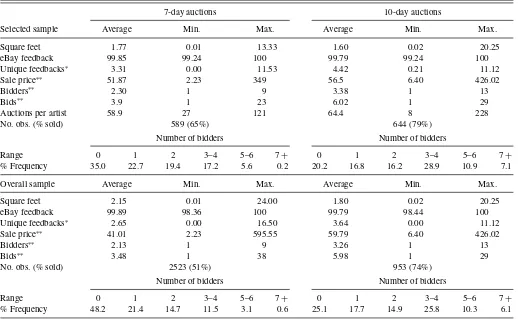
Table 2presents descriptive statistics for relevant variables
from the original sample and the selected subsample. The aver-age number of 7- and 10-day auctions among the 10 artists is 59 and 64, respectively. The artists in our subsample experience a higher average probability of sale, receive bids from a larger number of bidders, and have a more extensive eBay history, as indicated by the “unique feedback” variable. Auctions with zero bidders represent about 35% of auctions in the selected subsam-ple, auctions with two, three, or four bidders are not uncommon. Six percent of the auctions in the 7-day auctions category and 18% in the 10-day auctions had more than four active bidders. Multiple bids from single bidders are not uncommon. The av-erage size of a painting is close to two square-feet but there is a large variation in size. All artists’ in our sample enjoy an excel-lent eBay feedback rating, with an average rating of about 99.8. The average sale price is about $52 for 7-day auctions and about $57 for 10-day auctions, including shipping costs. The observed average number of bidders is 2.3 for 7-day auctions and 3.4 for 10-day auctions. Other relevant variables not included in this ta-ble are style (abstract, contemporary, etc.), medium (acrylic, pen and ink, etc.), and ground (stretch canvas, canvas panel, etc.). Descriptive statistics for these additional variables are available from the authors.
3.2 Empirical Framework
We apply the methodology described in Section2to the anal-ysis of auction outcomes and to the artists’ choice of auction length. This application underscores the relevance of a method-ology that considers the process of bidder arrival as well as the distribution of bidders’ valuations. It also underscores the flex-ibility of our methodology, which can easily be embedded into a more complex empirical framework.
We model the artists’ choice of a 7-day or 10-day auction and determine how auction characteristics influence the process of bidder arrival and the distribution of bidders’ valuations. The artist’s choice of auction length is a potentially complex de-cision that may depend on the artist’s expectations about the probability of a sale, the sale price, and the problem of in-ventory management, among others. We model this problem using a simple discrete choice framework where{Iij=1} rep-resents the 10-day auction choice on the part of the artist and is characterized as a standard logit model with associated prob-abilitypij=L(ij), whereLis the logistic CDF, and withij representing an index function that accounts for artists’ spe-cific fixed effects and unobserved heterogeneity. (In our empir-ical specification,ijtakes the formxij′æ+̺ηij.) We incorpo-rate the choice of auction length into the model described in Section2, and the contribution to the partial likelihood function
Table 2. Descriptive statistics for relevant variables
7-day auctions 10-day auctions
Selected sample Average Min. Max. Average Min. Max.
Square feet 1.77 0.01 13.33 1.60 0.02 20.25
eBay feedback 99.85 99.24 100 99.79 99.24 100
Unique feedbacks∗ 3.31 0.00 11.53 4.42 0.21 11.12
Sale price∗∗ 51.87 2.23 349 56.5 6.40 426.02
Bidders∗∗ 2.30 1 9 3.38 1 13
Bids∗∗ 3.9 1 23 6.02 1 29
Auctions per artist 58.9 27 121 64.4 8 228
No. obs. (% sold) 589 (65%) 644 (79%)
Number of bidders Number of bidders
Range 0 1 2 3–4 5–6 7+ 0 1 2 3–4 5–6 7+
% Frequency 35.0 22.7 19.4 17.2 5.6 0.2 20.2 16.8 16.2 28.9 10.9 7.1 Overall sample Average Min. Max. Average Min. Max.
Square feet 2.15 0.01 24.00 1.80 0.02 20.25
eBay feedback 99.89 98.36 100 99.79 98.44 100
Unique feedbacks∗ 2.65 0.00 16.50 3.64 0.00 11.12
Sale price∗∗ 41.01 2.23 595.55 59.79 6.40 426.02
Bidders∗∗ 2.13 1 9 3.26 1 13
Bids∗∗ 3.48 1 38 5.98 1 29
No. obs. (% sold) 2523 (51%) 953 (74%)
Number of bidders Number of bidders
Range 0 1 2 3–4 5–6 7+ 0 1 2 3–4 5–6 7+
% Frequency 48.2 21.4 14.7 11.5 3.1 0.6 25.1 17.7 14.9 25.8 10.3 6.1
NOTE: Sale price includes shipping costs.∗Measured in hundreds of feedbacks by unique buyers.∗∗Refers to sold paintings.
of a certain auctionjfrom artistiis described as
IijpijPL10ij +(1−Iij)(1−pij)PL7ij.
PL10
ij and PL7ijare the partial likelihood components defined by Equation (2) and are specific to 10-day and 7-day auctions.
Our econometric framework postulates an empirical specifi-cation governed by four equations: the artist’s choice of auction length, the process of bidders’ arrival (modeled as two sepa-rate Poisson processes, one for 10-day auctions and one for 7-day auctions), and the bidders’ valuation of the painting being auctioned (modeled as a single common equation for 7- and 10-day auctions). We experimented with other model specifica-tion structures, like a structure with a single bidder arrival equa-tion, but this specification was selected based on a likelihood-ratio-test criteria. Differences across auctions are captured by a vector of covariates as described in Section3.1. We also in-clude a dummy for year 2001 that captures any potential overall change in the market across years, biweekly dummies intended to capture seasonal effects on demand that are common across years, and a dummy variable intended to capture the potential impact of the terrorists attacks of 9/11 on auctions that took place in the weeks after this date. The empirical specification also includes artists’ specific fixed effects to account for unob-served differences across artists, in addition to those captured by the vector of covariates.
An unobserved heterogeneity component, as described in Section2, is incorporated into our empirical specification. We consider a distribution of unobserved heterogeneity with two points of support and with mean zero and variance one restric-tions. Baker and Melino (2000) showed that this specification
works well. (The estimated empirical distribution takes val-ues 0.905 and−1.357 with associated probabilities 0.628 and 0.372.) Estimation results are very similar for models with and without unobserved heterogeneity, and the coefficients asso-ciated to the unobserved heterogeneity are insignificant in all equations. However, a likelihood ratio test cannot reject the possible presence of unobserved heterogeneity.
In addition, the process of new bidders’ arrival includes a baseline hazard,λ(·), consisting of a constant and four additional baseline parameters. The first baseline parameter accounts for differences in the arrival of bidders between the second day and the day before the end of the auction; the second, third, and fourth baselines account for differences in the rate of arrival on the last day, the last hour, and the last 10 min of the auction, respectively. The arrival process also includes dummies for the day of the week in which the auction ends, allowing for the possible changes in the flow of potential buyers at different days of the week. Some variables are included in the bidder-arrival equation but not in the bidder-valuation equation. We hypothesize that bidders’ valuations are independent of day-of-the-week effects and other calendar dummies, which are more likely to affect the process of bidders’ arrival and have no direct effect on bidders’ valuation. These variables are insignificant when included in the bidders’ valuation equation.
3.3 Estimation Results
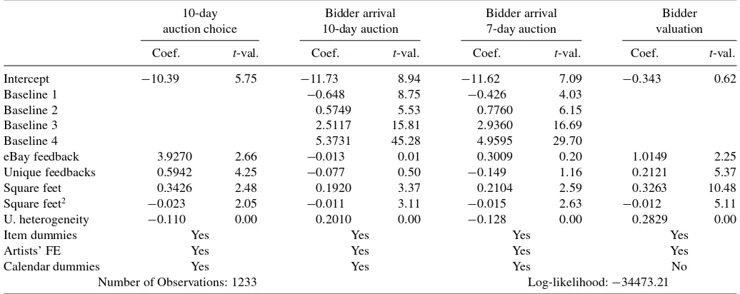
Table 3summarizes the most relevant estimation results. The
results from the bidder-valuation indicate that the most sig-nificant determinant of bidder-valuation is painting size, after
Table 3. Estimation results from model with unobserved heterogeneity
10-day Bidder arrival Bidder arrival Bidder auction choice 10-day auction 7-day auction valuation Coef. t-val. Coef. t-val. Coef. t-val. Coef. t-val. Intercept −10.39 5.75 −11.73 8.94 −11.62 7.09 −0.343 0.62
Baseline 1 −0.648 8.75 −0.426 4.03
Baseline 2 0.5749 5.53 0.7760 6.15
Baseline 3 2.5117 15.81 2.9360 16.69
Baseline 4 5.3731 45.28 4.9595 29.70
eBay feedback 3.9270 2.66 −0.013 0.01 0.3009 0.20 1.0149 2.25 Unique feedbacks 0.5942 4.25 −0.077 0.50 −0.149 1.16 0.2121 5.37 Square feet 0.3426 2.48 0.1920 3.37 0.2104 2.59 0.3263 10.48 Square feet2
−0.023 2.05 −0.011 3.11 −0.015 2.63 −0.012 5.11 U. heterogeneity −0.110 0.00 0.2010 0.00 −0.128 0.00 0.2829 0.00
Item dummies Yes Yes Yes Yes
Artists’ FE Yes Yes Yes Yes
Calendar dummies Yes Yes Yes No
Number of Observations: 1233 Log-likelihood:−34473.21
NOTE: Item dummies indicate item specific dummies for style, medium, and ground types. U. heterogeneity stands for unobserved heterogeneity and Artists’ FE stands for artists’ fixed effects.
controlling for other factors including artists’ fixed effects. An increase in one square foot in size increases a bidder’s valuation by 30% on average. Interestingly, both measures of seller’s feed-back are significant. An increase in 100 unique previous buyers increases bidders’ valuation by 21%. Possible interpretations are that this represents a reputation effect or that this measures the increase in sellers’ intrinsic value as a result of learning-by-doing. Two possible learning-by-doing channels are improve-ments in technique or gaining a better understanding of what characteristics of the artwork bidders’ value the most. In particu-lar, we observe an increase in the average painting size overtime, which is consistent with the artists learning about bidders’ tastes. The average impact of a decrease in eBay feedback rating of 0.1, for example, from 99.8 to 99.7, will result in a relatively large decrease in average bidders’ valuation of 10.1%.
Our results contrast with reported findings of the cross-sectional literature in this area. Bajari and Hortac¸su (2003) found that a negative reputation does not significantly impact the final auction price. Melnik and Alm (2002) estimated that the impact of negative feedback is significant but very small in magnitude, and the same holds for the impact of the overall rating. Houser and Wooders (2006) estimated that the average cost to sellers stemming from neutral or negative reputation scores is less than one percent (0.93%) of the final sales price. Lucking-Reiley et al. (2007) estimated that a one percent increase in positive/negative feedback increases/reduces sale price by only 0.03% and 0.11%, respectively. Bajari and Hortac¸su (2004) reviewed this evidence and concluded: “We believe that these results are likely to sig-nificantly understate the returns from having a good reputation . . .Since getting positive feedback requires effort on the part of sellers, it appears that sellers are making efforts to avoid negative feedback. . ..” The estimated effect in our case is much larger than what has been reported in existing cross-sectional studies. With regard to the bidder-arrival process, we observe again that size has a significant positive effect. Interestingly, reputation measures have an insignificant impact on bidders’ arrival rates, with the exception of the “number of feedbacks” variable that is
significant for the 7-day bidder-arrival process. Thus, reputation does not seem to play a significant role in the arrival of bidders for the group of sellers considered in our analysis. The baseline hazard coefficients associated to the bidder-arrival equations are similar across 7- and 10-day auctions. The baseline hazard coefficients, “Baseline 3” and “Baseline 4,” are larger and more significant indicating that bidders are more likely to arrive later in the auction. The first and second baselines are somewhat larger for the 7-day auction arrival process, indicating a lower bidder arrival rate between the first and the last day of the auction in 10-day auctions.
Looking at the equation that models the choice of auction length, both the painting size and the seller reputation measures are significant. We view this as an interesting novel result which indicates that the measures of seller reputation have a significant effect not only on the valuations of bidders but also on the ac-tions of the sellers. However, while bidder arrival and valuation equations are identified from the choices of a large number of independent bidders, the choice of 10-day auctions is identified from the actions of the subgroup of 10 different sellers. Thus, it is warranted to analyze to what extent the findings about the choice of auction length also holds in the larger population of artists in the larger dataset. With this purpose in mind, we es-timate a conditional logit model in the larger sample with the same specification and controlling for artist’s specific fixed ef-fects. The results from this exercise are comparable to those from our structural estimation. The coefficients associated with the first and the second measure of reputation are 3.92 and 0.59, respectively, and are significant with associatedt-values 2.7 and 4.3, respectively. These values represent relatively large effects taking into account that the proportion of 10-day auctions is 27% in the large sample.
3.4 Counter-Factual Analysis
In addition to examining what factors influence the choice of auction length, we conduct a counter-factual analysis
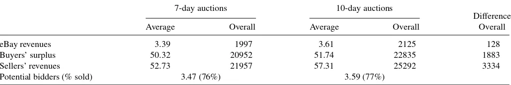
Table 4. Simulated market outcomes for two auction lengths
7-day auctions 10-day auctions
Difference Average Overall Average Overall Overall
eBay revenues 3.39 1997 3.61 2125 128
Buyers’ surplus 50.32 20952 51.74 22835 1883
Sellers’ revenues 52.73 21957 57.31 25292 3334
Potential bidders (% sold) 3.47 (76%) 3.59 (77%)
NOTE: Characteristics of each 7-day auction in our selected subsample are used for simulation. Simulated values are generated using average results from 100 draws from the estimated model. Seller revenues represent gross values before fees to eBay.
simulating what would happen if 7-day auctions were instead listed as 10-day auctions. (We thank an anonymous referee for suggesting this application.) This analysis highlights the value of our structural model and estimates the impact of auction length on market outcomes such as sellers’ revenue, buyers’ surplus, and the revenue of the market intermediary.
The bidders’ arrival component of our structural model allows us to determine the impact of changes in auction length on the number of potential bidders in an auction. Similarly, the bidders’ valuation component of our structural model is applied, along with the implied changes in the number of potential bidders, to ascertain the impact of a change in auction length in the final transaction price. The final transaction price has an impact on sellers’ revenue, the revenue of the market intermediary, and the buyers’ surplus. Changes in the value of these factors as a result of changes in the auction length can be analyzed within the proposed structural framework.
We conduct our experiment assuming that the estimated structural model represents an accurate description of the data-generating process. For each 7-day auction in our selected sub-sample, we generate 100 realizations of potential outcomes re-sulting from posting an item with the same characteristics in an auction of a specific length and consider the average outcome from the simulation.
Simulation results for the average outcome for 7- and 10-day auctions are presented inTable 4. The first two columns present results for 7-day auctions, the next two columns present results under an alternative 10-day scenario, and in the final column, we report the difference in overall outcomes. We observe that the number of potential bidders is similar across auction formats but about 3% higher for 10-day auctions. This is consistent with our prior results concerning the bidder’s arrival process in 7-and 10-day auctions, which suggests a higher intensity of bid-der arrival in 7-day auctions, especially toward the end of the auction. Average seller revenues are $52.7 and $57.3 for 7- and 10-day auctions. The simulated revenues for 7-day auctions are in line with what we observe in the data but the simulations pre-dict a higher sales rate for 7-day auctions than what we observe in the data (76% predicted vs. 65% observed from Table 2). (In our analysis, we employed several parametric assumptions for simplicity, but our general approach is not reliant on the-ses assumptions. Thus, the model fit could potentially improve by experimenting with different semiparametric techniques and model specifications. This is potentially an avenue for further research, but beyond the current scope of the article.) Compar-ing simulation results for the second highest and highest bids, we compute the average buyer surplus. Buyer surplus is $50 and
$52 for 7- and 10-day auctions, respectively. Finally, examin-ing the list of fees applied by eBay, we approximately compute eBay’s revenues for 7- and 10-day auctions. Our results indicate that eBay revenues are $128 (6%) higher for 10-day auctions.
4. CONCLUSIONS
This article presents a novel structural approach for the esti-mation of IPV, ascending-bid, second-price auctions, the most popular type of auction mechanism used on Internet markets. Unlike previous studies, our estimation approach makes use of information on the time of arrival of bids, which is readily avail-able on eBay, along with information on bids from all auction participants. Both the arrival of bidders and the distribution of bidders’ valuations are modeled explicitly. In addition, we also take into account the specific features of eBay auctions: the number of potential bidders is a stochastic function of the auc-tion characteristics, and not all potential bids and bidders are observed. Our approach avoids potential problems of selection bias present in existing studies.
Estimation is performed by maximizing a partial likelihood function. While our estimated model includes a number of para-metric functional form assumptions, it is possible to use semi-parametric model specifications instead. We leave this for future work. We apply our methodology to the analysis of the artist’s choice of auction length (7- or 10-day auctions) and to the de-termination of auction outcomes in general. This application underscores the flexibility of our methodology, which can be easily embedded into a more complex empirical framework.
Our analysis indicates that painting size is an important determinant of bidder’s valuation and bidder’s participation in an auction. We also consider the effect of two measures of seller’s reputation and find that reputation has a significant effect on bidders valuations. The estimated effect is much larger than what has been reported in existing cross-sectional studies. In contrast, the impact of a seller’s reputation on bidder’s auction participation is to a large extent insignificant.
Interestingly when we consider the seller’s choice of auction length, our analysis indicates that a seller’s reputation has a significant effect on this choice. We find that a seller with a better reputation is more likely to choose an auction with a longer duration, thus a seller’s reputation impacts not only the choices of bidders but the choices of sellers as well. Our counter-factual analysis indicates that if sellers were to list 7-day auctions as 10-day auctions, the number of potential bidders would slightly increase and seller revenues would increase by 9%.
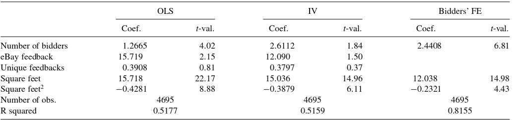
Table A.1 Regression of bid value on the number of bidders
OLS IV Bidders’ FE
Coef. t-val. Coef. t-val. Coef. t-val. Number of bidders 1.2665 4.02 2.6112 1.84 2.4408 6.81 eBay feedback 15.719 2.15 12.090 1.50
Unique feedbacks 0.3908 0.81 0.3797 0.37
Square feet 15.718 22.17 15.036 14.96 12.038 14.98
Square feet2 −0.4281 8.88 −0.3879 6.11 −0.2321 4.43
Number of obs. 4695 4695 4695
R squared 0.5177 0.5159 0.8155
NOTE: All models include controls for style, medium, ground, and artists’ fixed effects. The last model also controls for bidders’ fixed effects.
APPENDIX: TESTS OF INDEPENDENT PRIVATE VALUES
In the main body of the article, we present qualitative argu-ments supportive of the IPV assumption, while in this appendix, we formally test the IPV versus common value (CV) assump-tion. We rely on tests that have been applied by researchers in prior studies. Existing tests to distinguish IPV models from CV models are based on the winner’s curse (Paarsch1992; Bajari and Hortac¸su2003; Haile, Hong, and Shum2003). In CV auc-tions, bidders lower their bids in expectation of the winner’s curse and the amount bids are lowered is a function of the num-ber of observed bidders. The winner’s curse does not apply to the IPV paradigm where there is no signaling component to additional observed bidders.
We use IPV/CV tests similar to those used by Bajari and Hortac¸su (2003) and present a novel test taking advantage of the unique panel structure of our dataset. The tests we use regress bidders’ highest bids on the number of bidders in the auction and other auction characteristics. Under the CV (IPV) paradigm, we would expect to observe a negative (positive) coefficient associated to the number of bidders variable. [The coefficient for the number of bidders is expected to be positive for IPV due to the truncation from the eBay auction format. See footnote 16 of Bajari and Hortac¸su (2003) and theorem 9 of Athey and Haile (2002).]
The tests we use distinguish a pure CV model from an IPV model. These tests do not distinguish between IPV and an inter-dependent private values model. Haile, Hong, and Shum (2003) developed a test to distinguish between IPV and interdependent values with unobserved heterogeneity and endogenous entry, but this test is only relevant for first price auctions rather than the second-price auctions considered here. Additionally, in practice, it may be difficult to distinguish an interdependent private val-ues model from a model of unobserved heterogeneity. Given the very limited role that unobserved heterogeneity plays in the re-sults from our structural model, we feel that the IPV assumption is not inappropriate for our application.
Table A.1presents results from our IPV/CV tests for the
over-all sample of auctions with two or more bidders. The first model presents results from a simple ordinary least squares (OLS) regression that includes controls for relevant painting charac-teristics (i.e., style, medium, and ground) as well as artists’ reputation and artists’ fixed effects. Observable characteristics in our sample explain a large proportion of the variation in
final auction prices. Furthermore, our structural analysis sug-gests that unobserved heterogeneity plays a very limited role. Thus, we feel confident that the OLS specification of the test provides relevant information. Furthermore, a second model considers an IV approach that includes a battery of calendar dummies (i.e., day of the week and month) as instruments for the number of bidders, which should account for changes in demand but should not affect bidders’ valuations directly, after controlling for the number of bidders in an auction. These vari-ables are insignificant when included in our structural analysis in the bidders’ valuation equation. One potential problem with the previous two tests is that they do not take into account the potential effect of differences in bidders’ tastes. To control for this confounding effect, one needs a panel data that includes re-peated observations of bids for the same bidders, which we have in our data. The coefficients associated with seller’s reputation and with painting size have the expected sign for all models with the exception of the last one which does not include controls for seller’s reputation because there is no sufficient remaining vari-ation to identify these coefficients with any level of precision. The coefficient associated to the number of bidders is positive in all models and ranges from $1.2 to $2.6. This coefficient is significant at the usual level for the first and third model, while it is significant at the 90% level for the second model. These results are supportive of the IPV paradigm.
SUPPLEMENTARY MATERIALS
The online supplementary Appendix evaluates the robustness of our modeling assumptions, discusses identification of the model, describes eBay auctions, and expands further on the relevance of the data set to our application.
ACKNOWLEDGMENTS
For useful comments, we thank Robert McNown, the edi-tors Arthur Lewbel, Keisuke Hirano, and Jonathan Wright, an associate editor, two referees, and seminar participants at the University of Colorado and participants at the following confer-ences: Conference in Tribute to Jean-Jacques Laffont, Toulouse, May 2005; The 75th Southern Economic Association Meetings; The XXX Simposio de Analisis Economico; The Midwest Eco-nomic Association Meetings, April 2006; The Summer Meet-ings of the Econometric Society, June 2006; and The Midwest
Econometrics Group Meetings, October 2006. Excellent edito-rial assistance was provided by Katrina Beck. Excellent research assistance was provided by David Donofrio, Tyson Gatto, and especially Woong Tae Chung and Kelvin Tang. We are grateful to Kristen Stein, artist and eBay power seller, for answering many questions on the functioning of eBay and on bidders’ and artists’ behavior. Canals-Cerd´a gratefully acknowledges fund-ing from a CARTSS (Center for Advanced Research and Teach-ing in the Social Sciences) small grant from the University of Colorado. These are the views of the authors and should not be attributed to any other person or organization, including the Federal Reserve Bank of Philadelphia.
[Received November 2006. Revised October 2012.]
REFERENCES
Ackerberg, D., Hirano, K., and Shahriar, Q. (2006), “The Buy-It-Now Option, Risk Aversion, and Impatience in an Empirical Model of eBay Bidding,” Working Paper, University of Arizona. [126,128,129]
Athey, S., and Haile, P. A. (2002), “Identification of Standard Auction Models,” Econometrica, 70, 2107–2140. [134]
——— (2007), “Nonparametric Approaches to Auctions,” inHandbook of Econometrics(Vol. 6A), eds. J. J. Heckman and E. Leamer, Amsterdam: Elsevier. [126]
Bajari, P., and Hortac¸su, A. (2003), “The Winner’s Curse, Reserve Prices, and Endogenous Entry: Empirical Insights From eBay Auctions,”The RAND Journal of Economics, 34, 329–355. [125,126,132,134]
——— (2004), “Economic Insights From Internet Auctions,”Journal of Eco-nomic Literature, XLII, 457–486. [126,132]
Baker, M., and Melino, A. (2000), “Duration Dependence and Nonparametric Heterogeneity: A Monte Carlo Study,”Journal of Econometrics, 96, 357– 393. [131]
Baldwin, L. H., Marshall, R. C., and Richard, J. F. (1997), “Bidder Collusion and Forest Service Timber Sales,”Journal of Political Economy, 105, 657– 699. [125]
Cameron, A. C., and Trivedi, P. (1998), “Regression Analysis of Count Data,” (Econometric Society Monograph) (Vol. 30), Cambridge: Cambridge Uni-versity Press. [128]
Canals-Cerd´a, J. J. (2005), “Congestion Pricing in an Internet Market,” Working Paper 05-10, NET Institute. [125]
——— (2006), “Advertising as a Signal in an Internet Auctions Market,” avail-able athttp://ssrn.com/abstract=935093. [125]
Donald, S. G., and Paarsch, H. J. (1996), “Identification, Estimation and Testing in Parametric Empirical Models of Auctions Within the Independent Private Values Paradigm,”Econometric Theory, 12, 517–567. [125]
Flinn, C., and Heckman, J. J. (1982), “New Methods for Analyzing Struc-tural Models of Labor Force Dynamics,” Journal of Econometrics, 18, 115–168. [127]
Haile, P. A. (2001), “Auctions With Resale Markets: An Application to U.S. Forest Service Timber Sales,”American Economic Review, 91, 399–427. [125]
Haile, P. A., Hong, H., and Shum, M. (2003), “Nonparametric Tests for Common Values at First-Price Sealed Bid Auctions,” Working Paper 10105, National Bureau of Economic Research. [134]
Haile, P. A., and Tamer, E. T. (2003), “Inference With an Incomplete Model of English Auctions,”Journal of Political Economy, 111, 1–51. [125,127] Heckman, J. J., and Singer, B. (1984), “A Method for Minimizing the Impact
of Distributional Assumptions in Econometric Models for Duration Data,” Econometrica, 52, 271–320. [129]
Heckman, J. J., and Walker, J. R. (1990), “The Relationship Between Wages and Income and the Timing and Spacing of Births: Evidence From Swedish Longitudinal Data,”Econometrica, 58, 1411–1441. [128]
Hendricks, K., and Paarsch, H. J. (1995), “A Survey of Recent Empiri-cal Work Concerning Auctions,” Canadian Journal of Economics, 28, 403–426. [125]
Hong, H., and Shum, M. (2003), “Econometric Models of Asymmetric Ascend-ing Auctions,”Journal of Econometrics, 112, 327–358. [125]
Houser, D., and Wooders, J. (2006), “Reputation in Auctions: Theory, and Evidence From eBay,”Journal of Economics and Management Strategy, 15, 353–369. [132]
Lancaster, T. (1990),The Econometric Analysis of Transition Data. New York: Cambridge University Press. [128]
Lucking-Reiley, D. (2000), “Auctions on the Internet: What’s Being Auctioned, and How?”Journal of Industrial Economics, 48, 227–252. [125,126] Lucking-Reiley, D., Bryan, D., Prasad, N., and Reeves, D. (2007), “Pennies
From eBay: The Determinants of Price in Online Auctions,”The Journal of Industrial Economics, 55, 223–233. [132]
Melnik, M., and Alm, J. (2002), “Does a Seller’s eCommerce Reputation Matter? Evidence From eBay Auctions,”The Journal of Industrial Economics, 50, 337–349. [132]
Meyer, B. (1990), “Unemployment Insurance and Unemployment Spells,” Econometrica, 58, 757–782. [128]
Milgrom, P. R., and Weber, R. J. (1982), “A Theory of Auctions and Competitive Bidding,”Econometrica, 50, 1089–1122. [125]
Paarsch, H. J. (1992), “Empirical Models of Auctions and an Application to British Columbian Timber Sales,” Research Report no. 9212, University of Western Ontario, London. [125,134]
——— (1997), “Deriving an Estimate of the Optimal Reserve Price: An Ap-plication to British Columbian Timber Sales,”Journal of Econometrics, 78, 333–357. [125]
Song, U. (2004), “Nonparametric Estimation of an eBay Auction Model With an Unknown Number of Bidders,” Working Paper, University of Wisconsin at Madison. [126]
Villas-Boas, S. B. (2006), “An Introduction to Auctions,”Journal of Industrial Organization Education, 1, 5. [128]
Wang, R. (1993), “Auctions Versus Posted-Price Selling,”The American Eco-nomic Review, 83, 838–851. [127]