Optimal Design of Parmameters for Digital
Controllers Using Nonlinear Programing Technique
Le Hoa Nguyen
Department of Electrical Engineering, Danang University of Science and Technology-The Unversity of Danang
Danang, Vietnam Email: [email protected]
Demi Soetraprawata, Arjon Turnip
Technical Implementation Unit for InstrumentationDevelopment, Indonesia Institute of Science Bangdung, Indonesia
Email: [email protected]
Abstract—This paper presents a method to optimal design of parameters for digital controllers using a nonlinear programming technique. Firstly, the performance index and constraint functions in terms of controller’s parameters are derived and formulated as a nonlinear programming problem. Then the penalty function approach is proposed as an optimization algorithm to solve the nonlinear programming problem, where the constrained optimization problem is transformed into a series of unconstrained optimization problems. Finally, the efficiency of the proposed method is illustrated through an example of optimal design parameter for a digital controller of a simple plant.
Keywords— Nonlinear programming; penalty function; SUMT; PI controller (key words).
I. INTRODUCTION
In the field of control engineering, it is always required the control system operates as close as possible on the optimal trajectory. Several methods have been proposed to find the optimal trajectory of a control system such as Pontryagin’s
minimum principle, Bellman’s dynamic programming method, etc. [1]. In order to guarantee the system operates stably as close as possible on the optimal trajectory, a controlled will be designed. Steps to design a controller includes i) select an appropriate structure for the controller and ii) find suitable parameters for the controller. Finding suitable controller’s parameters depends on the performance index of the control systems, such as short settling time, small overshoot, small value of the squared error, etc. In this paper we will focus on determination of optimal parameters for the controller with assume that the controller’s structure is known. Traditional
controller’s parameters design methods mainly base on the experience of the designer. In some special cases, empirical rules can be applied to find the controller’s parameters [2]. However, there is no general procedure to design the controller’s parameters from given system’s specifications. Therefore, it is possible to use the performance index function formulated in terms of controller’s parameters to describe the desired performance of the control system. In addition, the designed controller must satisfy some equality constraints as well as inequality constraints with respect to the controller’s parameters. These constraints may come from the requirements of the stability of the system, the limitation of control signal, etc. Generally, the performance index function
along with constraints can be formulated as a nonlinear programming problem.
In this paper, the penalty method approach is proposed to solve a nonlinear programming problem. The advantage of the penalty method is it can transform a constrained optimization problem into a series of unconstrained optimization problems. The efficiency of the proposed method is illustrated through an example of optimal design parameter for a digital controller of a simple plant.
II. FORMULATION THE METHOD
A. Nonlinear Programing Problem
As mentioned above, for a given system’s specification,
one can use the performance index function in terms of
controller’s parameters to describe the desired performance of
the system. Suppose that it is required to minimize the following performance index function.
) (x F
J (1)
where x
x1 x2 xn
Tis a variable vector with respectto the controller’s parameters. Furthermore, suppose that the
parameters of the controller are constrained such that the following inequality and equality should be satisfied.
p i
x
gi( )0, 0,1,, (2)
q j
x
hj( )0, 0,1,, (3)
where, gi(x) and hj(x) present inequality constraints and
equality contraints, respectively.
Then, the desired performance and constraints in term of the
controller’s parameters can be formulated as follows
n j
i
R X x
q j x
h
p i x g
x F J
, , 0 , 0 ) (
, 0 , 0 ) (
min ) (
(4)
The problem described by (4) is called a nonlinear programming problem.
The set
( )0, ( )0
x Xg x h x
D i j (5)
is called a constraint set (or feasible region). Every point
2015 International Conference on Automation, Cognitive Science, Optics, Micro Electro-Mechanical System, and Information Technology (ICACOMIT), Bandung, Indonesia, October 29–30, 2015
x x x
Dx 1 2 n T is called a feasible solution. A
solution x*D is called an optimal solution if and only if the following condition is satisfied
x F
x x DF * , . (6)
B. Penalty Method Approach
One possible method for solving the problem described by (4) is the penalty method [3, 7]. The idea of a penalty method is to transform a constrained optimization problem into a series of unconstrained optimization problem by adding penalty terms such that the solution of unconstrained optimization problem converges to the solution of the original constrained optimization problem. This technique is also known as sequential unconstrained minimization technique (SUMT) according to the work of Fiacco and McCormick. [4, 5].
General transformation of constrained problem given by (4) into an unconstrained problem is as follows
min ) ( )
( )
(
k x F x Rk k x , (7)
where Rk is a scalar denoted as the penalty or controlling
parameter, Ψk(x) is the penalty function (note that Ψk(x) is
controlled by Rk), Φk(x) is the (pseudo) transformed objective
function. Ψk(x) and a sequence Rk must be chosen such that
when k goes to infinity, the solution of (7) exits and converges to the solution of (4) as fast as possible.
In this paper, the penalty function Ψk(x) is proposed as
follows
q
j j j k p
i
p i
i i k i
i k
k h x
R x g R x g R x
1 2
1 1
2
) ( 1
) ( 1
) ( )
(
, (8)where Rk is chosen such that it satisfies the following
condition
0 k
R and lim 0
k
k
R . (9)
In order to guarantee the solution of (7) converges to the solution of (4), the parameters
i,
i, and
j are chosen such that they satisfy the following conditions
0 ) ( if 0 and 0
0 ) ( if 0 and 0
, 0
x g
x g
i i
i
i i
i j
(10)
The process for finding the optimal solution of the unconstrained optimization problem described by (7)-(10) is summarized as follows
(1) Starting at an initial value of x . After k-2 iterations, we 0 obtain the value of xk1.
(2) Calculate the values of ( 1), j( k1)
k
i x h x
g and the values
of
i,
i, and
jaccording to (10). (3) Find the solution xkof (7).(4) Verifying the error of the solution at every iteration as follows
k k
k
1
1 ,k k
k F
2F , (11)
k k
k F F
F 1
3 .where,Fk,Fk1are the values of the cost function at kth
and(k1)th iteration, respectively. k, k1are the values of
the transformed objective function atkth
and(k1)thinteraction, respectively.
1, 2, 3 are the admissible errors.(5) Stop if the conditions described by (10) satisfied,
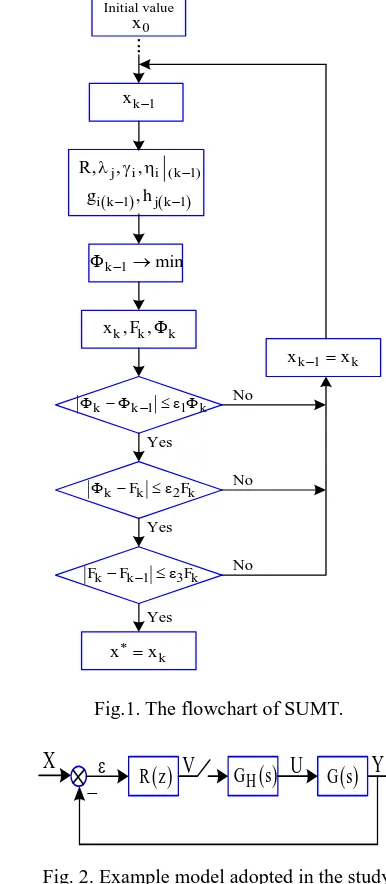
otherwise, setxk1bexkand return to the step 2. The flowchart of SUMT is described as in Fig. 1.
III. EXAMPLE
In this part, a numerical example is taken to illustrate the idea of the above mentioned method. The example shows how to find optimal parameters for a PI digital controller of a SISO system. The model adopted in this study is shown in Fig. 2.
0
x
Initial value
k 1
x
j i i (k 1)
R, , ,
i k 1 j k 1
g , h
k 1 min
k k k
x , F ,
k k 1 1 k
k Fk 2 kF
k k 1 3 k
F F F
k
xx
k 1 k
x x
..
.
Yes Yes Yes
No
No
[image:2.595.144.509.252.740.2]No
Fig.1. The flowchart of SUMT. .
X
V
U
Y
R z GH
s G s
[image:2.595.323.516.274.716.2]where, G(s) is a transfer function of the plant and it is selected as follows ) 5 )( 1 ( 625 . 0 ) )( ( ) ( 2
1
s s s s s s k s
G . (12)
GH(s) is the transfer function of the zero-order hold
sT e s G sT H 1 )
( . (13)
R(z) is a transfer function of the PI digital controller, given as
1 0 1 1 1 ( ) 1
a a z
R z b z
. (14)
Problem statement: Determination of optimal parameters for
the controller (a0, a1, b1) such that the system is stable and the
settling time of a transient response is minimal.
From Fig. 2 and (12)-(14), the following relationships can be obtained.
( ). ( )
( ) ( )
1 ( ). ( ) GH z R z
Y z X z
GH z R z
. (15)
1
( ) ( )
1 ( ) ( )
z X z
GH z R z
. (16)
( )
( ) ( )
1 ( ) ( )
R z
V z X z
GH z R z
. (17)
where, GH(z)is the transfer function of G(s) and GH(s) in
z-domain, and it is obtained as follows
0 1 2 2 1 1 ) )( ( 1 ) ( g z g z B z A s s s s s k Z z zGH k k
. (18)
where 1 2 2 1 1 2 2 1 2 1 2 1 2 1 2 1 2 1 ) 1 ( ) 1 ( ) ( , ) ( , ) ( , 2 1 Ct Bt t At B t C t B t t A A e t e t s s s k C s s s k B s s k A k k T s T s (19)
where T is the sampling time.
Finally, we obtain the following relationships
2
2 1 0
3 2
2 1 0
( ) u z u z u ( )
Y z X z
z w z w z w
, (20)
3 2
2 1 0
3 2
2 1 0
( )z z v z v z v X z( )
z w z w z w
, (21)
3 2
2 1 0 0 1
3 2
1
2 1 0
( ) z v z v z v a z a ( )
V z X z
z b
z w z w z w
(22)
where
0 1
1 0 1
2 0
k
k k
k
u a B
u a B a A
u a A
,
0 1 0
1 0 1 1
2 1 1
v b c
v c b c
v g b
,
0 0 0
1 1 1
2 2 2
w v u
w v u
w v u
and c0 = t1t2, c1 = -(t1+t2).
A. Determine constraints
a) Constrain from the stability condition
Exponential stability criterion for the system is implemented by assignment 0 and 1 0 , 0
0
ze zT T
z T . (23)
where, α is called a decay coefficient.
The characteristic polynomial of the system is obtained as follows.
3 3 2 20 2 0 1 0 0
3 2
3 2 1 0
N z T z w T z w T z w
q z q z q z q
(24)
where q0 w q0; 1w t q1; 2w t2 2;q3t3.
By using Jury stability criterion, we obtain the following constraints.
3 2 1 0
3 2 1 0
3 0
2 2
0 3 0 2 3 1
0
( ) 0
0
0
q q q q
q q q q
q q
q q q q q q
(25)
Note that, (25) is derived from the stability condition of the system, when it is calculated on the computer in which the
equal sign “=” can be appeared, therefore, it is necessary to add a very small value
into (25) as follows3 2 1 0
3 2 1 0
3 0
2 2
0 3 0 2 3 1
0
( ) 0
0
0
q q q q
q q q q
q q
q q q q q q
(26)b) Constrain from the vanishing of steady error
Assume that the input signal is a unit step function, then
1 1 ( ) 1 X z z
. (27)
The steady error is required to be zero, therefore, by applying the final value theorem for discrete systems, we have
1 1
( ) lim(1 ) ( ) z
z z
. (28)
Substitution (21) and (27) into (28), finally we obtain 1
1
b . (29)
B. Cost function
The required performance of this system is to minimize the settling time of a transient response. Therefore, through the exponential stability criterion, a decay coefficient must be maximize or must be minimize as shown in the following equation
0 1
( , , ) min
F a a
(30)From the above equations, determining optimal parameters for the PI digital controller leads to solving a nonlinear programming problem described as follows
min ) (x
1 3 2 1 0
2 3 2 1 0
3 3 0
2 2
4 0 3 0 2 3 1
5
0
( ) 0
0
0
0
g x q q q q
g x q q q q
g x q q
g x q q q q q q
g x
(31)
C. Simulation result
In this section, the SUMT algorithms depicted in Fig. 1 is performed by using Matlab. Let choose the initial values such as
0
0 10, 20, 5.5, 4.6,1.5
T T
x a a
.After 85 iterations, the optimal values are obtained as follows
* * * *
1, 2, 15.3021, 13.3720,1.7818
T T
x a a
.
Here, the values of admissible error (
1, 2, 3) are chosen as6
1 2 3 10
.Therefore, the optimal PI digital controller is obtained as follows
1
1 15.3021 13.3720 ( )
1
z R z
z
.
Fig. 3, 4, 5 shows the step response of a system with the optimal parameters of a controller in comparison with the step response of an arbitrary set of parameters of the controller in the stable region (25).
0 1 2 3 4 5
0 0.2 0.4 0.6 0.8 1 1.2 1.4
Time [s]
stable response optimal response
Fig. 3. The output response (Y) of the system
0 1 2 3 4 5
0 5 10 15 20
Time[s]
stable response optimal response
0 1 2 3 4 5
-0.4 -0.2 0 0.2 0.4 0.6 0.8 1
Time[s]
[image:4.595.323.540.61.202.2]stable response optimal response
Fig. 5. The error response (ε) of the system.
IV. CONCLUSION
This paper presented a design method to optimize
controller’s parameters to achieve a desired performance by using a nonlinear programming technique. A penalty method approach was proposed to obtain the solution of the nonlinear programing problem. The proposed method can be applied for finding optimal parameters of any types of controller and is easy to implement. In order to illustrate the idea of method, an example is given. The simulation results show the efficiency of the proposed method.
References
[1] E. K. Donald, Optimal Control Theory-An Introduction, Prentice Hall, 1970.
[2] K. Ogata, Modern Control Engineering, New Jersey, Prentice Hall, 1996.
[3] A.F.K. Morales and J. Gutiérrez_García, “Penalty function methods for
constrained optimization with genetic algorithms: a statistical analysis,”
Proceedings of the Second Mexican International Conference on Artificial Intelligence, 2002.
[4] A.V. Fiacco and G.P. McCormick, “The sequential unconstrained minimization technique for nonlinear programming, a primal-dual
method,” Management Science, vol. 10, pp. 360-366, 1964.
[5] E. A. Smith and D. W. Coit, “Penalty function”, Section C 5.2 of Handbook of Evolutionary Computation, 1995.
[6] V.M. Becerra, “Solving optimal control problems with state constraints
using nonlinear programming and simulation tools,” IEEE transactions
on Education, vol. 47, no.3, pp. 377-384, 2004.
[7] M. Bazaraa, H. Sherali, and C.Shetty, “Nonlinear Programming: Theory and Algorithms”, New York: Wiley, 1993.
[8] C. Goh and K. Teo, “Control parametrization: A unified approach to
optimal control problems with general constraints,” Automatica, vol. 24,
[image:4.595.59.276.401.707.2]pp. 3-18, 1988.
![Fig. 4. The control signal (V) response of the systemTime[s]](https://thumb-ap.123doks.com/thumbv2/123dok/264509.506099/4.595.59.276.401.707/fig-control-signal-v-response-systemtime-s.webp)
