Chapter12 - Chi Square Tests and Nonparametric

(1)

Statistics for Managers

Using Microsoft® Excel

5th Edition

Chapter 12

(2)

Learning Objectives

In this chapter, you learn:



_{How and when to use the chi-square test for}

contingency tables



_{How to use the Marascuilo procedure for}

determining pair-wise differences when

evaluating more than two proportions

(3)

Contingency Tables



_{Useful in situations involving multiple}

population proportions



_{Used to classify sample observations}

according to two or more characteristics

(4)

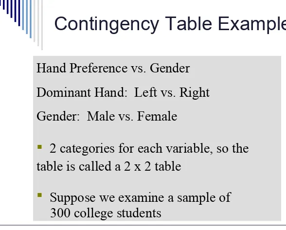
Contingency Table Example

Hand Preference vs. Gender

Dominant Hand: Left vs. Right

Gender: Male vs. Female



_{2 categories for each variable, so the}

table is called a 2 x 2 table



_{Suppose we examine a sample of}

(5)

Contingency Table Example

Sample results organized in a contingency table:

Hand

Preference

Gender

Female

Male

Left

12

24

36 Right

108

156

264

120

180

300 120 Females, 12 were

left handed

180 Males, 24 were

left handed

(6)

Contingency Table Example



_{If H}

₀

_{is true, then the proportion of left-handed females}

should be the same as the proportion of left-handed males.



_{The two proportions above should be the same as the}

proportion of left-handed people overall.

H

0 : π

1 = π

2 (Proportion of females who are left

handed is equal to the proportion of

males who are left handed)

H

1 : π

1 ≠ π

2 (The two proportions are not the same –

(7)

The Chi-Square Test Statistic

where:

f

o

= observed frequency in a particular cell

f

e

= expected frequency in a particular cell if H

0 is true



2 for the 2 x 2 case has 1 degree of freedom



cells

all

_e

2 e

o

2 f

)

f

(f

χ

The Chi-square test statistic is:

(8)

The Chi-Square Test Statistic

Decision Rule:

If

_

2 >

_

2 U

, reject H

0 ,

otherwise, do not reject

H

₀

The

_

2 test statistic approximately follows a chi-square

distribution with one degree of freedom



2 U

0 

Reject H

₀

Do not

(9)

Computing the

Average Proportion



_Here:

120 Females, 12 were

left handed

180 Males, 24 were

left handed

The proportion of left handers overall is 0.12, that is, 12%

n

The average

(10)

Finding Expected Frequencies



_{To obtain the expected frequency for left handed females,}

multiply the average proportion left handed (p) by the total

number of females



_{To obtain the expected frequency for left handed males,}

multiply the average proportion left handed (p) by the total

number of males

If the two proportions are equal, then

P(Left Handed | Female) = P(Left Handed | Male) = .12

i.e., we would expect

(.12)(120) = 14.4 females to be left handed

(11)

Observed vs. Expected

Frequencies

Hand

Preference

Gender

Female

Male

Left

Observed = 12

Expected = 14.4

Observed = 24

Expected = 21.6

36 Right

Observed = 108

Expected = 105.6

Observed = 156

Expected = 158.4

264

(12)

The Chi-Square Test Statistic

Hand

Preference

Gender

Female

Male

Left

Observed = 12

Expected = 14.4

Observed = 24

Expected = 21.6

36 Right

Observed = 108

Expected = 105.6

Observed = 156

Expected = 158.4

264

120

180

300 7576

(13)

The Chi-Square Test Statistic

Decision Rule:

If

_

2 > 3.841, reject H

conclude that there is

(14)



2 Test for The Differences Among

More Than Two Proportions



_{Extend the}

_

2 test to the case with more than two

independent populations:

H

0 : π

1 = π

2 = … = π

c

(15)

The Chi-Square Test Statistic

where:



_f

_o

_{= observed frequency in a particular cell of the 2 x c table}



_f

_e

_{= expected frequency in a particular cell if H}

₀

_{is true}



_

2 for the 2 x c case has (2-1)(c-1) = c - 1 degrees of freedom

Assumed: each cell in the contingency table has expected frequency of at

least 1



cells

all

2

2 (

)

e

o

f



(16)

Computing the

Overall Proportion

n

The overall

proportion is:



_{Expected cell frequencies for the c categories are}

calculated as in the 2 x 2 case, and the decision rule

is the same:

Decision Rule:

If

_

2 >

_

2 U

, reject H

0 ,

otherwise, do not

reject H

₀

Where

_

2 U

is from the

(17)



2 Test with More Than Two

Proportions: Example



_{The sharing of patient records is a}

controversial issue in health care. A survey

of 500 respondents asked whether they

objected to their records being shared by

insurance companies, by pharmacies, and by

medical researchers. The results are

(18)



2 Test with More Than Two

Proportions: Example

Object to

Record

Sharing

Organization

Insurance

Companies

Pharmacies

Medical

Researchers

Yes

410

295

335

(19)



2 Test with More Than Two

Proportions: Example

6933

The overall

proportion is:

Object to

Record

Sharing

Organization

Insurance

Companies

Pharmacies

Medical

Researchers

(20)



2 Test with More Than Two

Proportions: Example

Object

to

Record

Sharing

Organization

Insurance

Companies

Pharmacies

Medical

Researchers

Yes

(21)



2 Test with More Than Two

Proportions: Example

Decision Rule:

If



2 >



2 _U

, reject H

₀

,

otherwise, do not reject H

₀



2 _U

= 5.991 is from the

chi-square distribution with 2

degrees of freedom.

H

0 : π

1 = π

2 = π

3 H

1 : Not all of the π

j

are equal (j = 1, 2, 3)

Conclusion: Since 64.1196 > 5.991, you reject H

₀

and you

conclude that

at least one proportion of respondents who object to

their records being shared is different across the three

(22)

The Marascuilo Procedure

The

Marascuilo procedure

enables you to

make comparisons between all pairs of

groups.

First, compute the observed differences p

_j

- p

_j’

among all c(c-1)/2 pairs.

(23)

The Marascuilo Procedure



_{Critical Range for the Marascuilo Procedure:}

/

Critical

2

(24)

The Marascuilo Procedure



_{Compute a different critical range for each}

pair-wise comparison of sample proportions.



_{Compare each of the}

_{c(c -}

_{1)/2 pairs of}

sample proportions against its corresponding

critical range.



_{Declare a specific pair significantly different}

if the absolute difference in the sample

(25)

The Marascuilo Procedure

Example

Object to

Record

Sharing

Organization

Insurance

Companies

Pharmacies

Medical

Researchers

Yes

410 P

₁

= 0.82

295 P

₂

= 0.59

335 P

₃

= 0.67

(26)

The Marascuilo Procedure

Example

MARASCUILO TABLE

Proportions

Differences Critical Range

Absolute

| Group 1 - Group 2 |

0.23 0.06831808

| Group 1 - Group 3 |

0.15 0.0664689

| Group 2 - Group 3 |

0.08 0.074485617

Conclusion: Since each absolute difference is greater

than the critical range, you conclude that each

(27)



2 Test of Independence



_{Similar to the}

_

2 test for equality of more than two

proportions, but extends the concept to contingency

tables with r rows and c columns

H

0 : The two categorical variables are independent

(i.e., there is no relationship between them)

H

1 : The two categorical variables are dependent

(28)



2 Test of Independence



_where:

f

o

= observed frequency in a particular cell of the r x c table

f

e

= expected frequency in a particular cell if H

0

is true



2

for the r x c case has (r-1)(c-1) degrees of freedom

Assumed: each cell in the contingency table has expected

frequency of at least 1)



cells

all

_e

2 e

o

2 f

)

f

(

(29)

Expected Cell Frequencies



_{Expected cell frequencies:}

n

al

column tot

total

row

_



e

f

Where:

(30)

Decision Rule



_{The decision rule is}

If

_

2 >

_

2 U

, reject H

0 ,

otherwise, do not reject H

₀

(31)

Example: Test of Independence



_{The meal plan selected by 200 students is shown below:}

Class

Standing

Number of meals per week

Total

20/week

10/week

none

Fresh.

24

32

14

70 Soph.

22

26

12

60 Junior

10

14

6

30 Senior

14

16

10

40

(32)

Example: Test of Independence



_{The hypothesis to be tested is:}

H

0 : Meal plan and class standing are independent

(i.e., there is no relationship between them)

H

1 : Meal plan and class standing are dependent

(33)

Example: Test of Independence

Class

Standing

Number of meals

per week

Total

20/wk

10/wk

none

Fresh.

24.5

30.8

14.7

70 Soph.

21.0

26.4

12.6

60 Junior

10.5

13.2

6.3

30 Senior

14.0

17.6

8.4

40 Total

70

88

42

200 Expected cell frequencies

if H

₀

is true:

column tot

x

(34)

Example: Test of Independence



_{The test statistic value is:}

(35)

Example: Test of

Independence

Decision Rule:

If

_

2 > 12.592, reject H

statistic

test

The

_

2 _

_

_U

2 _

Here,



2 = 0.709 <



2 U

= 12.592,

so do not reject H

₀

Conclusion: there is

insufficient evidence that meal

plan and class standing are

(36)

McNemar Test



_{Used to test for the difference between two}

proportions of related samples (not

independent)



_{You need to use a test statistic that follows}

(37)

McNemar Test

Contingency Table

Condition (Group) 1

Condition (Group) 2

Yes

No

Totals

Yes

A

B

A+B

No

C

D

C+D

Totals

A+C

B+D

n

(38)

McNemar Test

Contingency Table

The sample proportions are:

Condition (Group) 1

Condition (Group) 2

Yes

No

Totals

Yes

A

B

A+B

No

C

D

C+D

Totals

A+C

B+D

n

C

A

p

n

B

A

(39)

McNemar Test

Contingency Table

The population proportions are:

π

₁

= proportion of the population who answer yes to condition 1

π

₂

= proportion of the population who answer yes to condition 2

Condition (Group) 1

Condition (Group) 2

Yes

No

Totals

Yes

A

B

A+B

No

C

D

C+D

(40)

McNemar Test

Test Statistic

To test the hypothesis:

H

₀

: π

₁

= π

₂

H

₁

: π

₁

≠ π

₂

Use the test statistic:

C

B

C

B

Z

(41)

McNemar Test

Example



_{Suppose you survey 300 homeowners and ask}

them if they are interested in refinancing their

home. In an effort to generate business, a

mortgage company improved their loan terms and

reduced closing costs. The same homeowners

(42)

McNemar Test

Example

Survey response

before change

Survey response after change

Yes

No

Totals

Yes

118

2

120 No

22

158

180 Totals

140

160

300 Test the hypothesis (at the 0.05 level of significance):

(43)

McNemar Test

Example

Survey

response

before change

Survey response after

change

Yes

No

Totals

Yes

118

2

120 No

22

158

180 Totals

140

160

300 The critical value (.05

significance) is Z = -1.96

The test statistic is:

(44)

Wilcoxon Rank-Sum Test



_{Test two independent population medians}



_{Populations need not be normally distributed}



_{Distribution free procedure}

(45)

Wilcoxon Rank-Sum Test



_{Can use when both n}

₁

_{, n}

₂

_{≤ 10}



_{Assign ranks to the combined n}

₁

_{+ n}

₂

_{sample values}



_{If unequal sample sizes, let n}

₁

_{refer to smaller-sized}

sample



_{Smallest value rank = 1, largest value rank = n}

₁

_{+ n}

₂



_{Assign average rank for ties}



_{Sum the ranks for each sample: T}

₁

_{and T}

₂

(46)

Checking the Rankings



_{The sum of the rankings must satisfy the formula}

below



_{Can use this to verify the sums T}

₁

_{and T}

₂

2 1)

n(n

2

1 



T

(47)

Wilcoxon Rank-Sum Test

Hypothesis and Decision

H

₀

: M

₁

= M

₂

H

₁

: M

₁

≠ M

₂

H

₀

: M

₁

≤ M

₂

H

₁

: M

₁

> M

₂

H

₀

: M

₁

≥ M

₂

H

₁

: M

₁

< M

₂

Two-Tail Test

Left-Tail Test

Right-Tail Test

M

₁

= median of population 1; M

₂

= median of population 2

Reject

T

_1L

T

_1U

Reject

Do Not

Reject

T

_1L

Do Not Reject

T

_1U

Reject

Do Not Reject

Test statistic = T

₁

(Sum of ranks from smaller sample)

Reject H

₀

if T

₁

≤ T

_1L

or if T

₁

≥ T

_1U

(48)

Wilcoxon Rank-Sum Test

Example with Small Samples



_{Sample data are collected on the capacity rates}

(% of capacity) for two factories.



_{Are the median operating rates for two}

factories the same?



_{For factory A, the rates are 71, 82, 77, 94, 88}



_{For factory B, the rates are 85, 82, 92, 97}



_{Test for equality of the population medians}

(49)

Wilcoxon Rank-Sum Test

Example with Small Samples

Capacity

Rank

Factory A Factory B Factory A Factory B

71

1

77

2

82

3.5

82

3.5

85

5

88

6

92

7

94

8

97

9 Rank Sums:

20.5

24.5 Tie in 3

rd

and

4 th

places

Ranked

Capacity

(50)

Wilcoxon Rank-Sum Test

Example with Small Samples

Factory B has the smaller sample size, so the test

statistic is the sum of the Factory B ranks:

T

₁

= 24.5

The sample sizes are:

n

₁

= 4 (factory B)

(51)

Wilcoxon Rank-Sum Test

Example with Small Samples

n

₂



_n

₁

One-Tailed

Tailed

Two-

4

5

4

5 .05

.10

12, 28

19, 36

.025

.05

11, 29

17, 38

.01

.02

10, 30

16, 39

.005

.01

--, --

15, 40

6 

Lower and

Upper Critical

Values for T

₁

from

Appendix

Table E.8:

(52)

Wilcoxon Rank-Sum Test

Example with Small Samples

H

₀

: M

₁

= M

₂

H

₁

: M

₁

≠ M

₂

Two-Tail Test

Reject

T

_1L

=11

T

_1U

=29

Reject

Do Not

Reject

Reject H

₀

if T

₁

≤ T

_1L

= 11



_

_{= .05}



_n

₁

_{= 4 , n}

₂

_{= 5}

Test Statistic

_{from smaller sample):}

(Sum of ranks

T

₁

= 24.5

Decision:

Conclusion:

Do not reject at a = 0.05

(53)

Wilcoxon Rank-Sum Test

Using Normal Approximation



_{For large samples, the test statistic T}

₁

_{is approximately normal}

with mean and standard deviation:



_{Must use the normal approximation if either n}

₁

_{or n}

₂

_{> 10}



_{Assign n}

₁

_{to be the smaller of the two sample sizes}



_{Can use the normal approximation for small samples}

(54)

Wilcoxon Rank-Sum Test

Using Normal Approximation



_{The Z test statistic is}



_{Where Z approximately follows a standardized}

normal distribution

1

1 σ

μ

Z

1 T

T

_

(55)

Wilcoxon Rank-Sum Test

Using Normal Approximation

Use the setting of the prior example:

The sample sizes were:

n

₁

= 4 (factory B)

n

₂

= 5 (factory A)

The level of significance was α = .05

(56)

Wilcoxon Rank-Sum Test

Using Normal Approximation



_{The test statistic is}

20

(57)

Kruskal-Wallis Rank Test



_{Tests the equality of more than 2 population medians}



_{Use when the normality assumption for one-way}

ANOVA is violated



_Assumptions:



_{The samples are random and independent}



_{variables have a continuous distribution}



_{the data can be ranked}

(58)

Kruskal-Wallis Rank Test



_{Obtain overall rankings for each value}



_{In event of tie, each of the tied values gets the average}

rank



_{Sum the rankings for data from each of the c}

groups

(59)

Kruskal-Wallis Rank Test



_{The Kruskal-Wallis H test statistic:}

(with c – 1 degrees of freedom)

n = total number of values over the combined samples

c = Number of groups

T

_j

= Sum of ranks in the j

th

_sample

(60)

Kruskal-Wallis Rank Test



_{Decision rule}



_{Reject H}

₀

_{if test statistic H >}

_

_2U



_{Otherwise do not reject H}

₀



_{Complete the test by comparing the calculated H value}

to a critical

_

2 value from the chi-square distribution

with c – 1 degrees of freedom



2 U

0 

Reject H

₀

Do not

(61)

Kruskal-Wallis Rank Test

Example



_{Do different branch offices have a different number of}

employees?

Office size

(Chicago, C)

(Denver, D)

Office size

(Houston, H)

Office size

23

41

54

78

66

55

60

72

45

70

(62)

Kruskal-Wallis Rank Test

Example



_{Do different branch offices have a different}

number of employees?

Office size

(Chicago, C)

Ranking

Office size

(Denver, D)

Ranking

Class size

(Houston, H)

Ranking

(63)

Kruskal-Wallis Rank Test

Example



_{The H statistic is}

(64)

Kruskal-Wallis Rank Test

Example

Since H = 6.72

>

,

reject H

0

5.991

2 U



χ



_{Compare H = 6.72 to the critical value from the chi-square}

distribution for 3 – 1 = 2 degrees of freedom and

_

= .05:

There is evidence of a difference in the

population median number of employees in

the branch offices

5.991

2 U



(65)

Chapter Summary



_{Developed and applied the}

_

2 test for the difference between

two proportions



_{Developed and applied the}

_

2 test for differences in more than

two proportions



_{Examined the}

_

2 test for independence



_{Used the McNemar test for differences in two related}

proportions



_{Used the Wilcoxon rank sum test for two population medians}



_{Small Samples}



_{Large sample Z approximation}



_{Applied the Kruskal-Wallis H-test for multiple population}

medians