Valence Bond Methods. Theory and Applications G A Gallup

(1)

Valence Bond Methods

Theory and applications

(2)

VALENCE BOND METHODS Theory and applications

Valence bond theory is one of two commonly used methods in molecular quantum mechanics, the other is molecular orbital theory. This book focuses on the first of these methods,ab initiovalence bond theory.

The book is split into two parts. Part I gives simple examples of two-electron calculations and the necessary theory to extend these to larger systems. Part II gives a series of case studies of related molecule sets designed to show the nature of the valence bond description of molecular structure. It also highlights the stability of this description to varying basis sets. There are references to the CRUNCH computer program for molecular structure calculations, which is currently available in the public domain. Throughout the book there are suggestions for further study using CRUNCH to supplement discussions and questions raised in the text.

The book will be of primary interest to researchers and students working on molecular electronic theory and computation in chemistry and chemical physics.

(3)

(4)

VALENCE BOND METHODS

Theory and applications

(5)

PUBLISHED BY CAMBRIDGE UNIVERSITY PRESS (VIRTUAL PUBLISHING)

FOR AND ON BEHALF OF THE PRESS SYNDICATE OF THE UNIVERSITY OF

CAMBRIDGE

The Pitt Building, Trumpington Street, Cambridge CB2 IRP

40 West 20th Street, New York, NY 10011-4211, USA

477 Williamstown Road, Port Melbourne, VIC 3207, Australia

http://www.cambridge.org

© Gordon A. Gallup 2002

This edition © Gordon A. Gallup 2003

First published in printed format 2002

A catalogue record for the original printed book is available

from the British Library and from the Library of Congress

Original ISBN 0 521 80392 6 hardback

(6)

(7)

(8)

Preface

One senses that it is out of style these days to write a book in the sciences all on one’s own. Most works coming out today are edited compilations of others’ articles collected into chapter-like organization. Perhaps one reason for this is the sheer size of the scientific literature, and the resulting feelings of incompetence engendered, although less honorable reasons are conceivable. Nevertheless, I have attempted this task and submit this book on various aspects of what is calledab initiovalence bond theory. In it I hope to have made a presentation that is useful for bringing the beginner along as well as presenting material of interest to one who is already a specialist. I have taught quantum mechanics to many students in my career and have come to the conclusion that the beginner frequently confuses the intricacies of mathematical arguments with subtlety. In this book I have not attempted to shy away from intricate presentations, but have worked at removing, insofar as possible, the more subtle ones. One of the ways of doing this is to give good descriptions of simple problems that can show the motivations we have for proceeding as we do with more demanding problems.

This is a book on one sort of model or trial wave function that can be used for molecular calculations of chemical or physical interest. It is in no way a book on the foundations of quantum mechanics – there are many that can be recommended. For the beginner one can still do little better than the books by Pauling and Wilson[1] and Eyring, Walter, and Kimbal[2]. A more recent work is by Levine[3], and for a more “physicsish” presentation the book by Messiah[4] is recommended. These are a little weak on the practice of group theory for which Cotton[5] may serve. A more fundamental work on group theory is by Hammermesh[6]. Some further group theory developments, not to my knowledge in any other book, are in Chapter 5. Some of what we do with the theory of symmetric groups is based fairly heavily on a little book by Rutherford[7].

This is a book onab initiovalence bond (VB) theory. There is a vast literature on “valence bond theory” – much of it devoted to semiempirical and qualitative

(15)

xiv Preface

discussions of structure and reactivity of many chemical substances. It is not my purpose to touch upon any of this except occasionally. Rather, I will restrict myself principally to the results and interpretation of theab initioversion of the theory. It must be admitted thatab initioVB applications are limited to smaller systems, but we shall stick to this more limited goal. Within what practitioners callab initioVB theory there are, in broad terms, two different approaches.

rCalculations in which the orbitals used are restricted to being centered on only one atom of the molecule. They are legitimately called “atomic orbitals”. Treatments of this sort may have many configurations involving different orbitals. This approach may be considered a direct descendent of the original Heitler–London work, which is discussed in Chapter 2. rCalculations in which the orbitals range over two or more atomic centers in the molecule. Although the resulting orbitals are not usually called “molecular orbitals” in this context, there might be some justification in doing so. Within this group of methods there are subcategories that will be addressed in the book. Treatments of this sort usually have relatively few configurations and may be considered descendents of the work of Coulson and Fisher, which is discussed in Chapter 3.

Each of these two approaches has its enthusiasts and its critics. I have attempted an even-handed description of them.

At various places in the text there are suggestions for further study to supple-ment a discussion or to address a question without a currently known answer. The CRUNCH program package developed by the author and his students is available on the Web for carrying out these studies.1_{This program package was used for all}

of the examples in the book with the exception of those in Sections 2.2–2.6. I wish to thank Jeffrey Mills who read large parts of the manuscript and made many useful comments with regard to both style and clarity of presentation. Lastly, I wish to thank all of the students I have had. They did much to contribute to this subject. As time passes, there is nothing like a group of interested students to keep one on one’s toes.

Lincoln, Nebraska Gordon A. Gallup

November 2001

(16)

List of abbreviations

AO atomic orbital

CI configuration interaction

CRUNCH computational resource for understanding chemistry DZP double-zeta plus polarization

EGSO eigenvector guided sequential orthogonalization ESE electronic Schr¨odinger equation

GAMESS general atomic and molecular electronic structure system GGVB Goddard’s generalized valence bond

GUGA graphical unitary group approach HLSP Heitler–London–Slater–Pauling LCAO linear combination of atomic orbitals LMP least motion path

MCVB multiconfiguration valence bond

MO molecular orbital

MOCI molecular orbital configuration interaction RHF spin-restricted Hartree–Fock

ROHF spin-restricted open-shell Hartree–Fock SEP static-exchange potential

SCF self-consistent-field SCVB spin coupled valence bond UHF unrestricted Hartree–Fock

VB valence bond

(17)

(18)

Part I

(19)

(20)

1 Introduction

1.1 History

In physics and chemistry making a direct calculation to determine the structure or properties of a system is frequently very difficult. Rather, one assumes at the outset an ideal or asymptotic form and then applies adjustments and corrections to make the calculation adhere to what is believed to be a more realistic picture of nature. The practice is no different in molecular structure calculation, but there has developed, in this field, two different “ideals”and two different approaches that proceed from them.

The approach used first, historically, and the one this book is about, is called the valence bond (VB) method today. Heitler and London[8], in their treatment of the H2 molecule, used a trial wave function that was appropriate for two H atoms at long distances and proceeded to use it for all distances. The ideal here is called the “separated atom limit”. The results were qualitatively correct, but did not give a particularly accurate value for the dissociation energy of the H−H bond. After the initial work, others made adjustments and corrections that improved the accuracy. This is discussed fully in Chapter 2. A crucial characteristic of the VB method is that the orbitals of different atoms must be considered as nonorthogonal.

The other approach, proposed slightly later by Hund[9] and further developed by Mulliken[10] is usually called the molecular orbital (MO) method. Basically, it views a molecule, particularly a diatomic molecule, in terms of its “united atom limit”. That is, H2is a He atom (not a real one with neutrons in the nucleus) in which the two positive charges are moved from coinciding to the correct distance for the molecule.1 _{HF could be viewed as a Ne atom with one proton moved from the} nucleus out to the molecular distance, etc. As in the VB case, further adjustments and corrections may be applied to improve accuracy. Although the united atom limit is not often mentioned in work today, its heritage exists in that MOs are universally

1 _{Although this is impossible to do in practice, we can certainly calculate the process on paper.}

(21)

4 1 Introduction

considered to be mutually orthogonal. We touch only occasionally upon MO theory in this book.

As formulated by Heitler and London, the original VB method, which was easily extendible to other diatomic molecules, supposed that the atoms making up the molecule were in (high-spin)Sstates. Heitler and Rumer later extended the theory to polyatomic molecules, but the atomic S state restriction was still, with a few exceptions, imposed. It is in this latter work that the famous Rumer[11] diagrams were introduced. Chemists continue to be intrigued with the possibility of correlat-ing the Rumer diagrams with bondcorrelat-ing structures, such as the familiar Kekul´e and Dewar bonding pictures for benzene.

Slater and Pauling introduced the idea of using whole atomic configurations rather than S states, although, for carbon, the difference is rather subtle. This, in turn, led to the introduction of hybridization and the maximum overlap criterion for bond formation[1].

Serber[12] and Van Vleck and Sherman[13] continued the analysis and intro-duced symmetric group arguments to aid in dealing with spin. About the same time the Japanese school involving Yamanouchi and Kotani[14] published analyses of the problem using symmetric group methods.

All of the foregoing work was of necessity fairly qualitative, and only the smallest of molecular systems could be handled. After WWII digital computers became available, and it was possible to test many of the qualitative ideas quantitatively.

In 1949 Coulson and Fisher[15] introduced the idea of nonlocalized orbitals to the VB world. Since that time, suggested schemes have proliferated, all with some connection to the original VB idea. As these ideas developed, the importance of the spin degeneracy problem emerged, and VB methods frequently were described and implemented in this context. We discuss this more fully later.

As this is being written at the beginning of the twenty-first century, even small computers have developed to the point whereab initioVB calculations that required “supercomputers”earlier can be carried out in a few minutes or at most a few hours. The development of parallel “supercomputers”, made up of many inexpensive per-sonal computer units is only one of the developments that may allow one to carry out ever more extensiveab initioVB calculations to look at and interpret molecular structure and reactivity from that unique viewpoint.

1.2 Mathematical background

(22)

1.2 Mathematical background 5

to examine the implications of quantum mechanics for molecular structure, it was immediately clear that the lower symmetry, even in diatomic molecules, causes significantly greater difficulties than those for atoms, and nonlinear polyatomic molecules are considerably more difficult still. The mathematical reasons for this are well understood, but it is beyond the scope of this book to pursue these questions. The interested reader may investigate many of the standard works detailing the properties of Lie groups and their applications to physics. There are many useful analytic tools this theory provides for aiding in the solution of partial differential equations, which is the basic mathematical problem we have before us.

1.2.1 Schr¨odinger’s equation

Schr¨odinger’s space equation, which is the starting point of most discussions of molecular structure, is the partial differential equation mentioned above that we must deal with. Again, it is beyond the scope of this book to give even a review of the foundations of quantum mechanics, therefore, we assume Schr¨odinger’s space equation as our starting point. Insofar as we ignore relativistic effects, it describes the energies and interactions that predominate in determining molecular structure. It describes in quantum mechanical terms the kinetic and potential energies of the particles, how they influence the wave function, and how that wave function, in turn, affects the energies. We take up the potential energy term first.

Coulomb’s law

Molecules consist of electrons and nuclei; the principal difference between a molecule and an atom is that the latter has only one particle of the nuclear sort. Classical potential theory, which in this case works for quantum mechanics, says that Coulomb’s law operates between charged particles. This asserts that the potential energy of a pair of spherical, charged objects is

V(_|r1₋r2_|)₌ q1q2

|r1₋r2_| = q1q2

r12 , (1.1)

whereq1andq2are the charges on the two particles, andr12is the scalar distance between them.

Units

(23)

6 1 Introduction

Hartree’s atomic units are usually all we will need. These are obtained by as-signing mass, length, and time units so that the mass of the electron,me₌1, the electronic charge,_|e_{| =}1, and Planck’s constant, ¯h₌1. An upshot of this is that the Bohr radius is also 1. If one needs to compare energies that are calculated in atomic units (hartrees) with measured quantities it is convenient to know that 1 hartree is 27.211396 eV, 6.27508_×105_{cal/mole, or 2.6254935}_×₁₀6_{joule/mole. The reader} should be cautioned that one of the most common pitfalls of using atomic units is to forget that the charge on the electron is₋1. Since equations written in atomic units have nomes,es, or ¯hs in them explicitly, their being all equal to 1, it is easy to lose track of the signs of terms involving the electronic charge. For the moment, however, we continue discussing the potential energy expression in Gaussian units.

The full potential energy

One of the remarkable features of Coulomb’s law when applied to nuclei and electrons is its additivity. The potential energy of an assemblage of particles is just the sum of all the pairwise interactions in the form given in Eq. (1.1). Thus, consider a system with K nuclei, α₌1,2, . . ., K having atomic numbers Zα. We also consider the molecule to have N electrons. If the molecule is uncharged as a whole, then

Zα= N. We will use lower case Latin letters,i, j,k, . . ., to label electrons and lower case Greek letters,α, β, γ , . . ., to label nuclei. The full potential energy may then be written

V ₌

α<β

e2ZαZβ rαβ −

iα e2Zα

riα +

i<j e2

ri j. (1.2)

Many investigations have shown that any deviations from this expression that occur in reality are many orders of magnitude smaller than the sizes of energies we need be concerned with.2Thus, we consider this expression to represent exactly that part of the potential energy due to the charges on the particles.

The kinetic energy

The kinetic energy in the Schr¨odinger equation is a rather different sort of quantity, being, in fact, a differential operator. In one sense, it is significantly simpler than the potential energy, since the kinetic energy of a particle depends only upon what it is doing, and not on what the other particles are doing. This may be contrasted with the potential energy, which depends not only on the position of the particle in question, but on the positions of all of the other particles, also. For our molecular

(24)

1.2 Mathematical background 7

system the kinetic energy operator is

T _{= −} α

¯ h2 2Mα∇

2 α−

i ¯ h2 2me∇

2

i, (1.3)

whereMαis the mass of theαthnucleus.

The differential equation

The Schr¨odinger equation may now be written symbolically as

(T ₊V) ₌E, (1.4)

where E is the numerical value of the total energy, and is the wave function. When Eq. (1.4) is solved with the various constraints required by the rules of quantum mechanics, one obtains the total energy and the wave function for the molecule. Other quantities of interest concerning the molecule may subsequently be determined from the wave function.

It is essentially this equation about which Dirac[17] made the famous (or infa-mous, depending upon your point of view) statement that all of chemistry is reduced to physics by it:

The general theory of quantum mechanics is now almost complete, the imperfections that still remain being in connection with the exact fitting in of the theory with relativity ideas. These give rise to difficulties only when high-speed particles are involved, and are therefore of no importance in the consideration of atomic and molecular structure and ordinary chemical reactions. . ..The underlying physical laws necessary for the mathematical theory of a large part of physics and the whole of chemistry are thus completely known, and the difficulty is only that the exact application of these laws leads to equations much too complicated to be soluble. . ..

To some, with what we might call a practical turn of mind, this seems silly. Our mathematical and computational abilities are not even close to being able to give useful general solutions to it. To those with a more philosophical outlook, it seems significant that, at our present level of understanding, Dirac’s statement is appar-ently true. Therefore, progress made in methods of solving Eq. (1.4) is improving our ability at making predictions from this equation that are useful for answering chemical questions.

The Born–Oppenheimer approximation

(25)

8 1 Introduction

is frequently ambiguous. It can refer to two somewhat different theories. The first is the reference above and the other one is found in an appendix of the book by Born and Huang on crystal structure[19]. In the latter treatment, it is assumed, based upon physical arguments, that the wave function of Eq. (1.4) may be written as the product of two other functions

(ri,rα)₌φ(rα)ψ(ri,rα), (1.5) where the nuclear positionsrα given inψ are parameters rather than variables in the normal sense. Theφis the actual wave function for nuclear motion and will not concern us at all in this book. If Eq. (1.5) is substituted into Eq. (1.4), various terms are collected, and small quantities dropped, we obtain what is frequently called the Schr¨odinger equation for the electrons using the Born–Oppenheimer approximation

−h¯

2

2me

i

∇2

iψ+Vψ =E(rα )ψ, (1.6)

where we have explicitly observed the dependence of the energy on the nuclear positions by writing it as E(rα ). Equation (1.6) might better be termed the Schr¨odinger equation for the electrons using the adiabatic approximation[20]. Of course, the only difference between this and Eq. (1.4) is the presence of the nuclear kinetic energy in the latter. A heuristic way of looking at Eq. (1.6) is to observe that it would arise if the masses of the nuclei all passed to infinity, i.e., the nuclei become stationary. Although a physically useful viewpoint, the actual validity of such a procedure requires some discussion, which we, however, do not give.

We now go farther, introducing atomic units and rearranging Eq. (1.6) slightly,

−1₂

i

∇2 iψ−

iα Zα riαψ+

i<j 1 ri jψ+

α<β ZαZβ

rαβ ψ = Eeψ. (1.7) This is the equation with which we must deal. We will refer to it so frequently, it will be convenient to have a brief name for it. It is the electronic Schr¨odinger equation, and we refer to it as the ESE. Solutions to it of varying accuracy have been calculated since the early days of quantum mechanics. Today, there exist computer programs both commercial and in the public domain that will carry out calculations to produce approximate solutions to the ESE. Indeed, a program of this sort is available from the author through the Internet.3_{Although not as large as some of} the others available, it will do many of the things the bigger programs will do, as well as a couple of things they do not: in particular, this program will do VB calculations of the sort we discuss in this book.

(26)

1.3 The variation theorem 9

1.3 The variation theorem

1.3.1 General variation functions

If we write the sum of the kinetic and potential energy operators as the Hamiltonian operatorT ₊V ₌H, the ESE may be written as

H₌ E. (1.8)

One of the remarkable results of quantum mechanics is the variation theorem, which states that

W ₌ |H|

_| ≥ E0, (1.9)

where E0 is the lowest allowed eigenvalue for the system. The fraction in Eq. (1.9) is frequently called the Rayleigh quotient. The basic use of this result is quite simple. One uses arguments based on similarity, intuition, guess-work, or whatever, to devise a suitable function for. Using Eq. (1.9) then necessarily gives us an upper bound to the true lowest energy, and, if we have been clever or lucky, the upper bound is a good approximation to the lowest energy. The most common way we use this is to construct a trial function,, that has a number of parameters in it. The quantity, W, in Eq. (1.9) is then a function of these parameters, and a minimization of W with respect to the parameters gives the best result possible within the limitations of the choice for. We will use this scheme in a number of discussions throughout the book.

1.3.2 Linear variation functions

A trial variation function that has linear variation parameters only is an important special case, since it allows an analysis giving a systematic improvement on the lowest upper bound as well as upper bounds for excited states. We shall assume that φ1, φ2, . . . ,represents a complete, normalized (but not necessarily orthogonal) set of functions for expanding the exact eigensolutions to the ESE. Thus we write

₌

∞

i₌1

φiCi, (1.10)

where theCi are the variation parameters. Substituting into Eq. (1.9) we obtain W ₌

i j Hi jCi∗Cj

i j Si jCi∗Cj

, (1.11)

where

Hi j ₌φi|H|φj , (1.12)

(27)

10 1 Introduction

We differentiateW with respect to theC_i∗s and set the results to zero to find the minimum, obtaining an equation for eachC_i∗,

j

(Hi j ₋W Si j)Cj =0 ; i =1,2,. . . . (1.14)

In deriving this we have used the properties of the integralsHi j ₌ H_{j i}∗ and a similar result forSi j. Equation (1.14) is discussed in all elementary textbooks wherein it is shown that aCj =0 solution exists only if theW has a specific set of values. It is sometimes called thegeneralized eigenvalue problemto distinguish from the case whenSis the identity matrix. We wish to pursue further information about theWs here.

Let us consider a variation function where we have chosen n of the functions, φi. We will then show that the eigenvalues of the n-function problem divide, i.e., occur between, the eigenvalues of the (n₊1)-function problem. In making this analysis we use an extension of the methods given by Brillouin[21] and MacDonald[22].

Having chosennof theφfunctions to start, we obtain an equation like Eq. (1.14), but with onlyn_×nmatrices andnterms,

n

j=1

Hi j ₋W(n)Si j

C(n)_j ₌0 ; i ₌1,2, . . . ,n. (1.15)

It is well known that sets of linear equations like Eq. (1.15) will possess nonzero solutions for the C(n)_j s only if the matrix of coefficients has a rank less than n. This is another way of saying that the determinant of the matrix is zero, so we have

H−W(n)S

=0. (1.16)

When expanded out, the determinant is a polynomial of degreen in the variable W(n), and it has n real roots if H and S are both Hermitian matrices, and S is positive definite. Indeed, ifS were not positive definite, this would signal that the basis functions were not all linearly independent, and that the basis was defective. If W(n) takes on one of the roots of Eq. (1.16) the matrix H ₋W(n)S is of rank n₋1 or less, and its rows are linearly dependent. There is thus at least one more nonzero vector with componentsC(n)_j that can be orthogonal to all of the rows. This is the solution we want.

It is useful to give a matrix solution to this problem. We affix a superscript(n)_to emphasize that we are discussing a matrix solution fornbasis functions. SinceS(n) is Hermitian, it may be diagonalized by a unitary matrix,T ₌(T†)−1

T†S(n)T ₌s(n)₌diags₁(n),s₂(n), . . . ,sn(n)

(28)

where the diagonal elements ofs(n)are all real and positive, because of the Hermitian and positive definite character of the overlap matrix. We may construct the inverse square root ofs(n), and, clearly, we obtain

Ts(n)−1/2†S(n)Ts(n)−1/2₌ I. (1.18) We subject H(n)_{to the same transformation and obtain}

T

s(n)−1/2† H(n)T

s(n)−1/2

= _H¯(n)_, _(1.19)

which is also Hermitian and may be diagonalized by a unitary matrix,U.Combining the various transformations, we obtain

V†H(n)V ₌h(n)₌diagh(n)₁ ,h(n)₂ , . . . ,h(n)_n , (1.20)

V†S(n)V ₌ I, (1.21)

V ₌Ts(n)−1/2U. (1.22)

We may now combine these matrices to obtain the null matrix

V†H(n)V ₋V†S(n)V h(n)₌0, (1.23) and multiplying this on the left by (V†)−1₌U(s(n))1/2T gives

H(n)V ₋S(n)V h(n)₌0. (1.24)

If we write out thekth_{column of this last equation, we have} n

j₌1

H_{i j}(n)₋h(n)_k S_{i j}(n)Vj k ₌0 ; i ₌1,2, . . . ,n. (1.25)

When this is compared with Eq. (1.15) we see that we have solved our prob-lem, if C(n) is thekth column of V and W(n) is thekth diagonal element of h(n). Thus the diagonal elements of h(n) are the roots of the determinantal equation Eq. (1.16).

Now consider the variation problem withn₊1 functions where we have added another of the basis functions to the set. We now have the matrices H(n+1) and S(n+1), and the new determinantal equation

H(n+1)−W(n+1)S(n+1)

=0. (1.26)

We may subject this to a transformation by the (n₊1)_×(n₊1) matrix ¯

V ₌

V 0

(29)

12 1 Introduction

Thus Eq. (1.26) becomes

0₌

We modify the determinant in Eq. (1.30) by using column operations. Multiply the ithcolumn by

¯

H(n_{i n}+₊1)₁₋W(n+1)_S_¯(n+1) i n₊1 h(n)_i ₋W(n+1)

and subtract it from the (n₊1)th_{column. This is seen to cancel the}_ith_{row element} in the last column. Performing this action for each of the first n columns, the determinant is converted to lower triangular form, and its value is just the product of the diagonal elements,

(30)

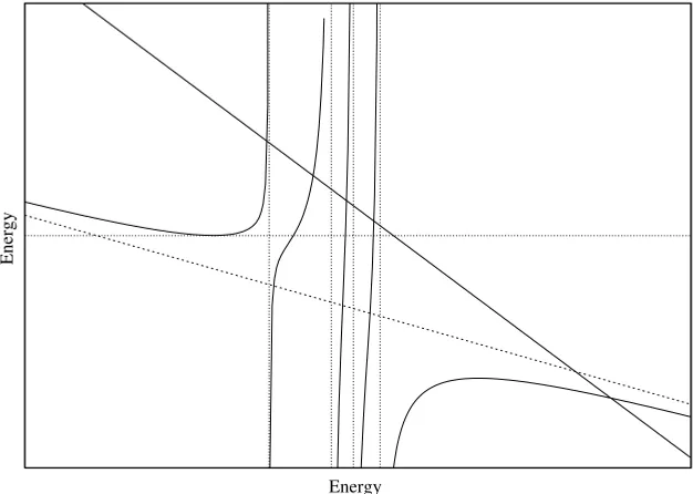
1.3 The variation theorem 13 It is most useful to consider the solution of Eq. (1.33) graphically by plotting both the right and left hand sides versus W(n+1) on the same graph and determining where the two curves cross. For this purpose let us suppose that n₌4, and we consider the right hand side. It will have poles on the real axis at each of theh(4)_i . WhenW(5)becomes large in either the positive or negative direction the right hand side asymptotically approaches the line

y₌

It is easily seen that the determinant of ¯Sis

|_S¯_{| =}₁₋

and, if equal to zero, S would not be positive definite, a circumstance that would happen only if our basis were linearly dependent. Thus, the asymptotic line of the right hand side has a slope between 0 and – 45◦. We see this in Fig. 1.1. The left hand side of Eq. (1.33) is, on the other hand, just a straight line of exactly – 45◦ slope and aW(5) _{intercept of ¯}_H(5)

5 5. This is also shown in Fig. 1.1. The important point we note is that the right hand side of Eq. (1.33) has five branches that in-tersect the left hand line in five places, and we thus obtain five roots. The vertical dotted lines in Fig. 1.1 are the values of theh(4)_i , and we see there is one of these between each pair of roots for the five-function problem. A little reflection will indicate that this important fact is true for anyn, not just the special case plotted in Fig. 1.1.

(31)

14 1 Introduction

Energy

Figure 1.1. The relationship between the roots forn₌4 (the abscissa intercepts of the vertical dotted lines) andn₌5 (abscissas of intersections of solid lines with solid curves) shown graphically.

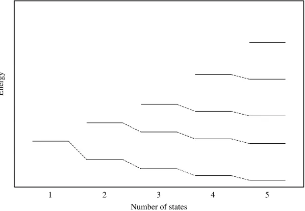
The upshot of these considerations is that a series of matrix solutions of the variation problem, where we add one new function at a time to the basis, will result in a series of eigenvalues in a pattern similar to that shown schematically in Fig. 1.2, and that the order of adding the functions is immaterial. Since we suppose that our ultimate basis (n_{→ ∞}) is complete, each of the eigenvalues will become exact as we pass to an infinite basis, and we see that the sequence of n-basis solutions converges to the correct answer from above. The rate of convergence at various levels will certainly depend upon the order in which the basis functions are added, but not the ultimate value.

1.3.3 A 2_×2 generalized eigenvalue problem

The generalized eigenvalue problem is unfortunately considerably more compli-cated than its regular counterpart whenS ₌I. There are possibilities for acciden-tal cases when basis functions apparently should mix, but they do not. We can give a simple example of this for a 2_×2 system. Assume we have the pair of matrices

H ₌

A B

(32)

Energy

Number of states

1 2 3 4 5

Figure 1.2. A qualitative graph showing schematically the interleaving of the eigenvalues for a series of linear variation problems forn ₌1, . . . ,5. The ordinate is energy.

and

S ₌

1 s

s 1 , (1.36)

where we assume for the argument thats >0. We form the matrixH′ H′ ₌H₋ A+C

2 S,

=

a b

b ₋a , (1.37)

where

a ₌ A₋ A+C

2 (1.38)

and

b₌ B₋ A+C

2 s. (1.39)

It is not difficult to show that the eigenvectors of H′are the same as those ofH. Our generalized eigenvalue problem thus depends upon three parameters, a, b, and s. Denoting the eigenvalue by W and solving the quadratic equation, we obtain

W _{= −} sb (1₋s2₎ ±

a2₍₁₋_s2₎₊_b2

(33)

16 1 Introduction

We note the possibility of an accident that cannot happen ifs ₌0 andb ₌0: Should b_{= ±}as, one of the two values ofW is either_±a, and one of the two diagonal elements of H′is unchanged.5_{Let us for definiteness assume that}_b

=asand it is awe obtain. Then, clearly the vectorC1we obtain is

1 0 ,

and there is no mixing between the states from the application of the variation theorem. The other eigenvector is simply determined because it must be orthogonal toC1, and we obtain

C2₌

−s/√1₋s2 1/√1₋s2 ,

so the other state is mixed. It must normally be assumed that this accident is rare in practical calculations. Solving the generalized eigenvalue problem results in a nonorthogonal basis changing both directions and internal angles to become orthogonal. Thus one basis function could get “stuck”in the process. This should be contrasted with the case when S₌ I, in which basis functions are unchanged only if the matrix was originally already diagonal with respect to them.

We do not discuss it, but there is an n_×n version of this complication. If there is no degeneracy, one of the diagonal elements of the H-matrix may be unchanged in going to the eigenvalues, and the eigenvector associated with it is [0, . . . ,0,1,0, . . . ,0]†.

1.4 Weights of nonorthogonal functions

The probability interpretation of the wave function in quantum mechanics obtained by forming the square of its magnitude leads naturally to a simple idea for the weights of constituent parts of the wave function when it is written as a linear combination of orthonormal functions. Thus, if

₌

i

ψiCi, (1.41)

andψi|ψj =δi j, normalization ofrequires

i

|Ci_|2₌1. (1.42)

If, also, each of the ψi has a certain physical interpretation or significance, then one says the wave function, or the state represented by it, consists of a fraction

(34)

1.4 Weights of nonorthogonal functions 17

|Ci_|2of the state represented byψi. One also says that theweight,wi ofψi inis wi = |Ci|2.

No such simple result is available for nonorthogonal bases, such as our VB functions, because, although they are normalized, they are not mutually orthogonal. Thus, instead of Eq. (1.42), we would have

i j

Ci∗CjSi j =1, (1.43)

if theψi were not orthonormal. In fact, at first glance orthogonalizing them would mix together characteristics that one might wish to consider separately in determin-ing weights. In the author’s opinion, there has not yet been devised a completely satisfactory solution to this problem. In the following paragraphs we mention some suggestions that have been made and, in addition, present yet another way of attempting to resolve this problem.

In Section 2.8 we discuss some simple functions used to represent the H2 mole-cule. We choose one involving six basis functions to illustrate the various methods. The overlap matrix for the basis is



0.962 004 1.000 000

0.137 187 0.181 541 1.000 000

−0.254 383 ₋0.336 628 0.141 789 1.000 000

0.181 541 0.137 187 0.925 640 0.251 156 1.000 000

0.336 628 0.254 383 ₋0.251 156 ₋0.788 501 ₋0.141 789 1.000 000

and the eigenvector we analyze is



S is to be filled out, of course, so that it is symmetric. The particular chemical or physical significance of the basis functions need not concern us here.

(35)

18 1 Introduction

Table 1.1.Weights for nonorthogonal basis functions by various methods.

Chirgwin– Inverse- Symmetric

Coulson overlap orthogon. EGSOa

0.266 999 0.106 151 0.501 707 0.004 998 0.691 753 0.670 769 0.508 663 0.944 675 –0.000 607 0.000 741 0.002 520 0.000 007 0.016 022 0.008 327 0.042 909 0.002 316 0.019 525 0.212 190 0.051 580 0.047 994 0.006 307 0.001 822 0.000 065 0.000 010

a_EGSO

=eigenvector guided sequential orthogonalization.

1.4.1 Weights without orthogonalization The method of Chirgwin and Coulson These workers[23] suggest that one use

wi =Ci∗

j

Si jCj, (1.45)

although, admittedly, they proposed it only in cases where the quantities were real. As written, thiswiis not guaranteed even to be real, and when theCiandSi jare real, it is not guaranteed to be positive. Nevertheless, in simple cases it can give some idea for weights. We show the results of applying this method to the eigenvector and overlap matrix in Table 1.1 above. We see that the relative weights of basis functions 2 and 1 are fairly large and the others are quite small.

Inverse overlapweights

Norbeck and the author[24] suggested that in cases where there is overlap, the basis functions each can be considered to have a unique portion. The “length”of this may be shown to be equal to the reciprocal of the diagonal of theS−1matrix corresponding to the basis function in question. Thus, if a basis function has a unique portion of very short length, a large coefficient for it means little. This suggests that a set ofrelativeweights could be obtained from

(36)

1.4.2 Weights requiring orthogonalization

We emphasize that here we are speaking of orthogonalizing the VB basis not the underlying atomic orbitals (AOs). This can be accomplished by a transformation of the overlap matrix to convert it to the identity

N†S N ₌ I. (1.47)

Investigation shows thatNis far from unique. Indeed, ifNsatisfies Eq. (1.47),N U will also work, whereU is any unitary matrix. A possible candidate forNis shown in Eq. (1.18). If we put restrictions on N, the result can be made unique. If N is forced to be upper triangular, one obtains the classicalSchmidt orthogonalization of the basis. The transformation of Eq. (1.18), as it stands, is frequently called thecanonical orthogonalizationof the basis. Once the basis is orthogonalized the weights are easily determined in the normal sense as

wi =

and, of course, they sum to 1 exactly without modification.

Symmetric orthogonalization

L¨owdin[25] suggested that one find the orthonormal set of functions that most closely approximates the original nonorthogonal set in the least squares sense and use these to determine the weights of various basis functions. An analysis shows that the appropriate transformation in the notation of Eq. (1.18) is

N ₌Ts(n)−1/2T† ₌S−1/2₌(S−1/2)†, (1.49) which is seen to be the inverse of one of the square roots of the overlap matrix and Hermitian (symmetric, if real). Because of this symmetry, using theNof Eq. (1.49) is frequently called asymmetric orthogonalization. This translates easily into the set of weights

(37)

20 1 Introduction

matrix were, in some sense, close to the identity would this method be expected to yield useful results.

An eigenvector guided sequential orthogonalization (EGSO)

As promised, with this book we introduce another suggestion for determining weights in VB functions. Let us go back to one of the ideas behind inverse overlap weights and apply it differently. The existence of nonzero overlaps between differ-ent basis functions suggests that some “parts”of basis functions are duplicated in the sum making up the total wave function. At the same time, consider function 2 (the second entry in the eigenvector (1.44)). The eigenvector was determined using linear variation functions, and clearly, there is something about function 2 that the variation theorem likes, it has the largest (in magnitude) coefficient. Therefore, we take all of that function in our orthogonalization, and, using a procedure analogous to the Schmidt procedure, orthogonalize all of the remaining functions of the basis to it. This produces a new set ofCs, and we can carry out the process again with the largest remaining coefficient. We thus have a stepwise procedure to orthogonalize the basis. Except for the order of choice of functions, this is just a Schmidt orthog-onalization, which normally, however, involves an arbitrary or preset ordering.

Comparing these weights to the others in Table 1.1 we note that there is now one truly dominant weight and the others are quite small. Function 2 is really a considerable portion of the total function at 94.5%. Of the remaining, only function 5 at 4.8% has any size. It is interesting that the two methods using somewhat the same idea predict the same two functions to be dominant.

If we apply this procedure to a different state, there will be a different ordering, in general, but this is expected. The orthogonalization in this procedure is not designed to generate a basis for general use, but is merely a device to separate characteristics of basis functions into noninteracting pieces that allows us to determine a set of weights. Different eigenvalues, i.e., different states, may well be quite different in this regard.

We now outline the procedure in more detail. Deferring the question of ordering until later, let us assume we have found an upper triangular transformation matrix, Nk, that convertsSas follows:

(Nk)†S Nk ₌

Ik 0 0 Sn₋k

, (1.51)

whereIkis ak_×kidentity, and we have determinedkof the orthogonalized weights. We show how to determineNk₊1fromNk.

(38)

elements equal to 1. We write it in partitioned form as

Sn₋k =

1 s

s† S′ , (1.52)

where [1 s] is the first row of the matrix. LetMn₋kbe an upper triangular matrix partitioned similarly,

Mn₋k =

1 q

0 B , (1.53)

and we determineq andBso that (Mn₋k)†Sn−kMn−k =

1 q ₊s B

(q₊s B)† B†(S′₋s†s)B , (1.54)

=

1 0

0 Sn₋k−1

, (1.55)

where these equations may be satisfied withBthe diagonal matrix

B₌diag1₋s₁2−1/21₋s₂2−1/2 _{· · ·} (1.56) and

q _{= −}s B. (1.57)

The inverse ofMn₋k is easily determined: (Mn₋k)−1=

1 s

0 B−1 , (1.58)

and, thus, Nk₊1=NkQk, where Qk ₌

Ik 0 0 Mn₋k

. (1.59)

The unreduced portion of the problem is now transformed as follows:

(Cn₋k)†Sn−kCn−k =[(Mn−k)−1Cn−k]†(Mn−k)†Sn−kMn−k[(Mn−k)−1Cn−k]. (1.60) Writing

Cn₋k =

C1

C′ , (1.61)

we have

[(Mn₋k)−1Cn₋k]=

C1₊sC′

B−1_C_′ , (1.62)

=

C1₊sC′ Cn₋k−1

. (1.63)

(39)

22 1 Introduction

What we have done so far is, of course, no different from a standard top-down Schmidt orthogonalization. We wish, however, to guide the ordering with the eigen-vector. This we accomplish by inserting before eachQka binary permutation matrix Pk that puts in the top position the C1₊sC′ from Eq. (1.63) that is largest in magnitude. Our actual transformation matrix is

N ₌ P1Q1P2Q2_{· · ·}Pn₋1Qn₋1. (1.64)

(40)

2 H

2

and localized orbitals

2.1 The separation of spin and space variables

One of the pedagogically unfortunate aspects of quantum mechanics is the com-plexity that arises in the interaction of electron spin with the Pauli exclusion prin-ciple as soon as there are more than two electrons. In general, since the ESE does not even contain any spin operators, the total spin operator must commute with it, and, thus, the total spin of a system of any size is conserved at this level of approximation. The corresponding solution to the ESE must reflect this. In addition, the total electronic wave function must also be antisymmetric in the interchange of any pair of space-spin coordinates, and the interaction of these two require-ments has a subtle influence on the energies that has no counterpart in classical systems.

2.1.1 The spin functions

When there are only two electrons the analysis is much simplified. Even quite elementary textbooks discuss two-electron systems. The simplicity is a conse-quence of the general nature of what is called thespin-degeneracy problem, which we describe in Chapters 4 and 5. For now we write the total solution for the ESE

(1,2), where the labels 1 and 2 refer to the coordinates (space and spin) of the two electrons. Since the ESE has no reference at all to spin,(1,2) may be factored into separate spatial and spin functions. For two electrons one has the familiar result that the spin functions are of either the singlet or triplet type,

1_φ 0=

η1/2(1)η−1/2(2)−η−1/2(1)η1/2(2)

√

2, (2.1)

3_φ

1=η1/2(1)η1/2(2), (2.2)

3_φ 0=

η1/2(1)η₋1/2(2)+η₋1/2(1)η1/2(2)

√

2, (2.3)

3_φ

−1=η₋1/2(1)η₋1/2(2), (2.4)

(41)

24 2 H2and localized orbitals

where on theφ the anterior superscript indicates the multiplicity and the posterior subscript indicates themsvalue. Theη_±1/2are the individual electron spin functions.

If we let Pi j represent an operator that interchanges all of the coordinates of the

ith_and _jth_{particles in the function to which it is applied, we see that}

P121φ0= −1φ0, (2.5)

P123φms = 3_φ

ms; (2.6)

thus, the singlet spin function is antisymmetric and the triplet functions are sym-metric with respect to interchange of the two sets of coordinates.

2.1.2 The spatial functions

The Pauli exclusion principle requires that the total wave function for electrons (fermions) have the property

P12(1,2)=(2,1)= −(1,2), (2.7)

but absence of spin in the ESE requires

(2S₊1)

ms(1,2)=

(2S₊1)_ψ₍₁_,₂₎

× (2S₊1)_φ

ms(1,2), (2.8)

and it is not hard to see that the overall antisymmetry requires that the spatial functionψ have behavior opposite to that ofφ in all cases. We emphasize that it is not an oversight to attach noms label toψin Eq. (2.8). An important principle in quantum mechanics, known as the Wigner–Eckart theorem, requires the spatial part of the wave function to be independent ofms for a givenS.

Thus the singlet spatial function is symmetric and the triplet one antisymmetric. If we use the variation theorem to obtain an approximate solution to the ESE requiring symmetry as a subsidiary condition, we are dealing with the singlet state for two electrons. Alternatively, antisymmetry, as a subsidiary condition, yields the triplet state.

We must now see how to obtain useful solutions to the ESE that satisfy these conditions.

2.2 The AO approximation

The only uncharged molecule with two electrons is H2, and we will consider this

(42)

2.2 The AO approximation 25

to be a normal H atom, for which we know the exact ground state wave function.1 The singlet wave function for this arrangement might be written

1

ψ(1,2)₌ N[1sa(1)1sb(2)+1sb(1)1sa(2)], (2.9) where 1saand 1sbare 1s orbital functions centered at nucleiaandb, respectively, andNis the normalization constant. This is just the spatial part of the wave function. We may now work with it alone, the only influence left from the spin is the “₊” in Eq. (2.9) chosen because we are examining the singlet state. The function of Eq. (2.9) is that given originally by Heitler and London[8].

Perhaps a small digression is in order on the use of the term “centered” in the last paragraph. When we write the ESE and its solutions, we use a single coordinate system, which, of course, has one origin. Then the position of each of the particles,

ri for electrons andrα for nuclei, is given by a vector from this common origin. When determining the 1sstate of H (with an infinitely massive proton), one obtains the result (in au)

1s(r)₌ _√1

π exp(−r), (2.10)

where r is the radial distance from the origin of this H atom problem, which is where the proton is. If nucleusα₌ais located atrathen 1sa(1) is a shorthand for

1sa=1s(|r1− ra|) = 1 √

π exp(−|r1− ra|), (2.11)

and we say that 1sa(1) is “centered at nucleusa”.

In actuality it will be useful later to generalize the function of Eq. (2.10) by changing its size. We do this by introducing a scale factor in the exponent and write

1s′(α,r)₌

α3

π exp(−αr). (2.12)

When we work out integrals for VB functions, we will normally do them in terms of this version of the H-atom function. We may reclaim the real H-atom function any time by settingα₌1.

Let us now investigate the normalization constant in Eq. (2.9). Direct substitution yields

1₌1ψ(1,2)_|1ψ(1,2) (2.13)

= |N_|2(1sa(1)|1sa(1)1sb(2)|1sb(2) + 1sb(1)|1sb(1)1sa(2)|1sa(2) + 1sa(1)|1sb(1)1sa(2)|1sb(2)

+ 1sb(1)|1sa(1)1sb(2)|1sa(2)), (2.14)

1 _{The actual distance required here is quite large. Herring[26] has shown that there are subtle effects due to}

(43)

where we have written out all of the terms. The 1s function in Eq. (2.10) is normalized, so

1sa(1)|1sa(1) = 1sb(2)|1sb(2), (2.15) = 1sb(1)|1sb(1), (2.16) = 1sa(2)|1sa(2), (2.17)

=1. (2.18)

The other four integrals are also equal to one another, and this is a function of the distance, R, between the two atoms called the overlap integral, S(R). The overlap integral is an elementary integral in the appropriate coordinate system, confocal ellipsoidal–hyperboloidal coordinates[27]. In terms of the function of Eq. (2.12) it has the form

S(w)₌(1₊w₊w2/3) exp(₋w), (2.19)

w₌αR, (2.20)

and we see that the normalization constant for1_ψ₍₁_,_{2) is}

N ₌[2(1₊S2)]−1/2. (2.21)

We may now substitute1ψ(1,2) into the Rayleigh quotient and obtain an estimate of the total energy,

E(R)₌1ψ(1,2)_|H_|1ψ(1,2)_≥ E0(R), (2.22)

whereE0is the true ground state electronic energy for H2. This expression involves

four new integrals that also can be evaluated in confocal ellipsoidal–hyperboloidal coordinates. In this case all are not so elementary, involving, as they do, expan-sions in Legendre functions. The final energy expression is (α₌1 in all of the integrals)

E ₌2h₋2j1(R)+S(R)k1(R) 1₊S(R)2 +

j2+k2

1₊S(R)2 +

1

R, (2.23)

where

h ₌α2/2₋α, (2.24)

j1= −[1−(1+w)e−2w]/R, (2.25)

k1= −α(1+w)e−w, (2.26)

j2=[1−(1+11w/8+3w2/4+w3/6)e−2w]/R, (2.27) k2= {6[S(w)2(C+lnw)−S(−w)2E1(4w)+2S(w)S(−w)E1(2w)]

(44)

2.4 Extensions to the simple Heitler–London treatment 27

Of these only the exchange integral of Eq. (2.28) is really troublesome to evaluate. It is written in terms of the overlap integral S(w), the same function of −w, S(−w)₌(1₋w₊w2/3)ew_{, the Euler constant,}_C

=0.577 215 664 901 532 86, and the exponential integral

E1(x)=

∞

x

e−yd y

y , (2.30)

which is discussed by Abramowitz and Stegun[28].

In our discussion we have merely given the expressions for the five integrals that appear in the energy. Those interested in the problem of evaluation are referred to Slater[27]. In practice, these expressions are neither very important nor useful. They are essentially restricted to the discussion of this simplest case of the H2molecule

and a few other diatomic systems. The use of AOs written as sums of Gaussian functions has become universal except for single-atom calculations. We, too, will use the Gaussian scheme for most of this book. The present discussion, included for historical reasons, is an exception.

2.3 Accuracy of the Heitler–London function

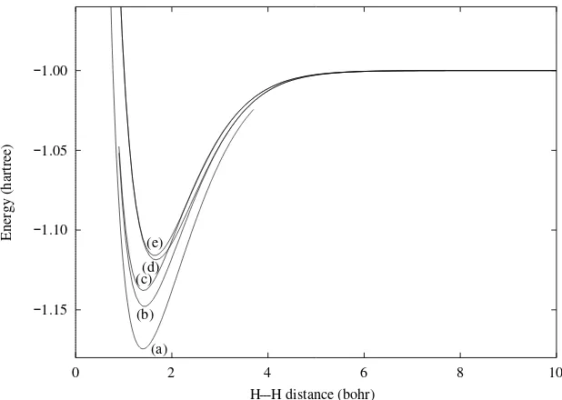
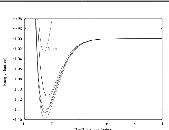
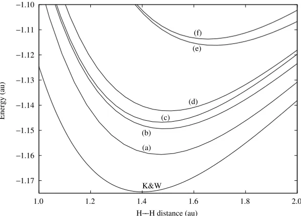
We are now in a position to compare our results with experiment. A graph ofE(R) given by Eq. (2.23) is shown as curve (e) in Fig. 2.1. As we see, it is qualitatively correct, showing the expected behavior of having a minimum with the energy rising to infinity at shorter distances and reaching a finite asymptote for large Rvalues. Nevertheless, it misses 34% of the binding energy (comparing with curve (a) of Fig. 2.1), a significant fraction, and its minimum is clearly at too large a bond distance.2

2.4 Extensions to the simple Heitler–London treatment

In the last section, our calculation used only the function of Eq. (2.9), what is now called the “covalent” bonding function. According to our discussion of linear variation functions, we should see an improvement in the energy if we perform a two-state calculation that also includes theionicfunction,

1_ψ

I(1,2)=N[1sa(1)1sa(2)+1sb(1)1sb(2)]. (2.31) When this is done we obtain the curve labeled (d) in Fig. 2.1, which, we see, represents a small improvement in the energy.

2 _{The quantity we have calculated here is appropriately compared to}_D_{e, the bond energy from the bottom of}

the curve. This differs from the experimental bond energy,D0, by the amount of energy due to the zero point

(45)

−1.15

−1.10

−1.05

−1.00

0 2 4 6 8 10

Energy (hartree)

H H distance (bohr) (e)

(d) (c)

(b)

(a)

---Figure 2.1. Energies of H2for various calculations using the H-atom 1sorbital functions; (b) covalent ₊ ionic, scaled; (c) covalent only, scaled; (d) covalent₊ ionic, unscaled; (e) covalent only, unscaled. (a) labels the curve for the accurate function due to Kolos and Wolniewicz[31]. This is included for comparison purposes.

A much larger improvement is obtained if we follow the suggestions of Wang[29] and Weinbaum[30] and use the 1s′(1) of Eq. (2.12), scaling the 1s H function at each internuclear distance to give the minimum energy according to the variation theorem. In Fig. 2.1 the covalent-only energy is labeled (c) and the two-state energy is labeled (b). There is now more difference between the one- and two-state energies and the better binding energy is all but 15% of the total.3 _{The scaling factor,}_α_,

shows a smooth rise from_≈1 at large distances to a value near 1.2 at the energy minimum.

Rhetorically, we might ask, what is it about the ionic function that produces the energy lowering, and just how does it differ from the covalent function? First, we note that the normalization constants for the two functions are the same, and, indeed, they represent exactly the same charge density. Nevertheless, they differ in their two-electron properties.1ψC(adding a subscriptCto indicate covalent) gives a higher probability that the electrons be far from one another, while 1ψI gives

3 _{Perhaps we should note that in this relatively simple case, we will approach the binding energy from below as}

(46)

2.4 Extensions to the simple Heitler–London treatment 29

just the opposite. This is only true, however, if the electrons are close to one or the other of the nuclei. If both of the electrons are near the mid-point of the bond, the two functions have nearly the same value. In fact, the overlap between these two functions is quite close to 1, indicating they are rather similar. At the equilibrium distance the basic orbital overlap from Eq. (2.19) is

S ₌1s_s′_|1s_{b =}′ 0.658 88. (2.32)

A simple calculation leads to

₌1ψC 1ψ_I

= 2S

1₊S2 =0.918 86. (2.33)

(We consider these relations further below.) The covalent function has been char-acterized by many workers as “overcorrelating” the two electrons in a bond. Presumably, mixing in a bit of the ionic function ameliorates the overage, but this does not really answer the questions at the beginning of this paragraph. We take up these questions more fully in the next section, where we discuss physical reasons for the stability of H2.

At the calculated energy minimum (optimumα) the total wave function is found to be

₌0.801 9811ψC +0.211 7021ψI. (2.34)

The relative values of the coefficients indicate that the variation theorem thinks better of the covalent function, but the other appears fairly high at first glance. If, however, we apply the EGSO process described in Section 1.4.2, we obtain 0.996 501ψC +0.083 541ψI′, where, of course, the covalent function is unchanged, but1ψ_I′is the new ionic function orthogonal to1ψC. On the basis of this calculation we conclude that the the covalent character in the wave function is (0.996 50)2₌ 0.993 (99.3%) of the total wave function, and the ionic character is only 0.7%.

(47)

Covalent Ionic

Eigenvector "Ionic" orthonormal vector

"Covalent" orthonormal vector (a)

(b)

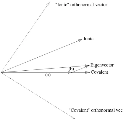
Figure 2.2. A geometric representation of functions for H2in terms of vectors forR=Req.

The small vectors labeled (a) and (b) are, respectively, the covalent and ionic components of the eigenvector. The vectors with dashed lines are the symmetrically orthogonalized basis functions for this case.

It is important to realize that the above geometric representation of the H2

Hilbert space functions is more than formal. The overlap integral of two normalized functions is a real measure of their closeness, as may be seen from

1

ψC− 1ψI

1ψ_C−1ψ_I

=2(1₋), (2.35)

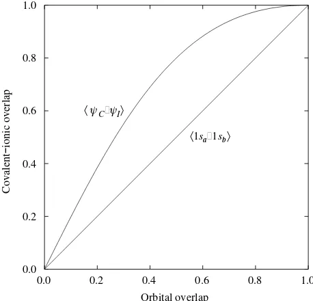
and, if the two functions were exactly the same, would be 1. As pointed out above,is a dependent uponS, the orbital overlap. Figure 2.3 shows the relation between these two quantities for the possible values ofS.

In addition, in Fig. 2.2 we have plotted with dashed lines the symmetrically orthogonalized basis functions in this treatment. It is simple to verify that

1

ψC−S1ψI

1ψ_I −S1ψ_C

=0, (2.36)