Parsimonious rainfall-runoff model construction supported by time
series processing and validation of hydrological extremes – Part 2:
Intercomparison of models and calibration approaches
q
Patrick Willems
⇑, Diego Mora, Thomas Vansteenkiste, Meron Teferi Taye, Niels Van Steenbergen
KU Leuven, Hydraulics Division, Kasteelpark Arenberg 40, BE-3001 Leuven, Belgium
a r t i c l e
i n f o
Article history:
Available online 21 January 2014
Keywords:
Hydrological extremes Lumped conceptual model Model calibration Rainfall-runoff
s u m m a r y
An intercomparison of different approaches for the construction and calibration of lumped conceptual rainfall-runoff models is made based on two case studies with unrelated meteorological and hydrological characteristics located in two regions, Belgium and Kenya. While a model with pre-fixed ‘‘one-size-fits-all’’ model structure is traditionally used in lumped conceptual rainfall-runoff modeling, this paper shows the advantages of model structure inference from data or field evidence in a case-specific and step-wise way using non-commensurable measures derived from observed series. The step-wise model structure identification method does not lead to higher accuracy than the traditional approach when evaluated using common statistical criteria like the Nash–Sutcliffe efficiency. The method is, however, favorable to produce a well-balanced calibration obtaining accurate results for a wide range of runoff properties: total flows, quick and slow subflows, cumulative volumes, peak flows, low flows, frequency distributions of peak and low flows, changes in quick flows for given changes in rainfall. It furthermore is shown that model performance evaluation procedures that account for the flow residual serial dependency and homoscedasticity are preferred. Explicit evaluation of model results for peak and/or low flow extremes and changes in these extremes make the models useful for impact investigations on such hydrological extremes.
Ó2014 The Authors. Published by Elsevier B.V. All rights reserved.
1. Introduction
Rainfall-runoff modelers have to face problems of data limita-tion. As a consequence of this limitation, they have to cope with several difficulties in model calibration. These include problems re-lated to model overparameterization, model parameter identifica-tion, and – when existing modeling softwares are applied – the validity of pre-defined process conceptualizations (Gupta and Sorooshian, 1983; Beven, 1993; Jakeman and Hornberger, 1993; Uhlenbrock et al., 1999; Perrin et al., 2001; among many others). There are several researchers who recently proposed solutions to meet one or more of these difficulties. Solutions range from the use of parsimonious conceptual models (to overcome the identifi-cation problem) to flexibility in setting the model structure (in-stead of using a pre-fixed model structure), the use of automated calibration methods and advanced or multiple objectives.Klemeš
(1983), Sivapalan et al. (2003)andSavenije (2009)are among the authors who explain why ‘‘top-down’’ or ‘‘downward’’ methods can compare favourably with the traditional approach based on parameter optimization of a given model with pre-fixed model structure. In top-down or downward methods, the model structure is adjusted or inferred from data or from field evidence. The use of multiple working hypotheses for testing of model alternatives was also promoted byClark et al. (2011). Recent developments in this direction include the flexible box models of Wagener et al. (2001) and the modular approach byFenicia et al. (2006, 2007). Other researchers developed advanced automated numerical parameter optimization methods (e.g. Duan et al., 1992; Vrugt et al., 2003) and/or calibration strategies based on multi-objectives where tradeoffs are made among different criteria (e.g.Gupta et al., 1998; Yapo et al., 1998; Boyle et al., 2000; Madsen, 2000; Madsen et al., 2002; Zhang et al., 2010). One of the challenges in this re-spect is the integration of ‘‘soft’’/‘‘qualitative’’ data or expert knowledge in the model building and calibration process.Seibert and McDonnell (2000) proposed to include expert knowledge as soft data in automatic calibration procedures by means of fuzzy measures of model performance. AlsoBormann (2011)used soft data (in the form of knowledge on surface shaping of a catchment) to verify and revise model parameterization. Question remains
0022-1694/$ - see front matterÓ2014 The Authors. Published by Elsevier B.V. All rights reserved. http://dx.doi.org/10.1016/j.jhydrol.2014.01.028
q
This is an open-access article distributed under the terms of the Creative Commons Attribution-NonCommercial-No Derivative Works License, which per-mits non-commercial use, distribution, and reproduction in any medium, provided the original author and source are credited.
⇑ Corresponding author. Tel.: +32 16 321658.
E-mail address:[email protected](P. Willems).
Contents lists available atScienceDirect
Journal of Hydrology
how far one should go in including such expert knowledge, given that it is subjective, hence difficult to objectify. Interesting is the conclusion byMadsen et al. (2002)that the use of generic search algorithms where user intervention is required only for the defini-tion of appropriate multi-objective numerical measures compare favourably with methods that require more user intervention and include subjective rules for trading off objectives.
This paper contributes to the above mentioned research challenges on the use of a top-down approach, the use of (tradeoff between) multiple objectives and the optimal use of expert knowl-edge. It starts from the approach presented byWillems (2014). This is a top-down approach to set a parsimonious lumped concep-tual rainfall-runoff model based on a multi-step model structure identification and calibration process. The approach aims to obtain a model valid for unbiased simulation of hourly or daily rainfall runoff for different components of flow and time scales that makes it applicable for studying hydrological extremes. In Willems (this isue), the approach was presented and demonstrated for a case study (Molenbeek river, Dender basin) in Belgium. Although the re-sults were accurate for that case study, and several advantages of the method postulated, comparison was not made with other methods. In this paper, the added value of the method is quanti-fied. It is tested whether the step-wise model identification and calibration procedure has advantages in comparison with tradi-tional approaches that involve model calibration of all parameters (of a pre-fixed model structure) based on overall goodness-of-fit optimization. In addition, the use of multiple objectives and the importance to account for the statistical assumptions and require-ments on independency and homoscedasticity of the model resid-uals is tested. This is done for two case studies in two regions with highly different meteorological and hydrological characteristics: the catchment of the Grote Nete river in Belgium, and the catch-ment of the Nyando river in the upper Nile basin in Kenya.
The paper is organized as follows. Section2outlines the meth-ods applied for testing the added value of the various aspects of the approach byWillems (2014). Section3introduces the two study catchments, followed by Section4with the results of the methods applied to these two catchments. Final conclusion and discussions are provided in Section5.
2. Methods
2.1. Step-wise model identification and calibration
The top-down procedure for lumped conceptual rainfall-runoff model building presented byWillems (2014)is hereafter denoted ‘‘VHM approach’’, according to a Dutch abbreviation. The final rainfall-runoff model obtained by that procedure is called VHM model.
The different VHM submodel process equations are identified and calibrated based on multiple subsets of non-commensurable information derived from river flow series by means of a number of sequential time series processing tasks. These include separation of the hourly or daily river flow series into subflows, split of the series in nearly independent quick and slow flow hydrograph peri-ods, and the extraction of approx. independent peak and low flows. Next to the separate identification of the subflow recessions and related routing submodels, equations describing quick and slow runoff sub-responses and soil water storage are derived from the river flow and rainfall time series data. The model building and cal-ibration, moreover, account for the statistical assumptions and requirements on independency and homoscedasticity of the model residuals. Model performance evaluation is based on peak and slow flow volumes as well as extreme high and low flow statistics, fol-lowing the method ofWillems (2009).
Whereas the final number of model parameters depends on the model structure identification process, the model structures obtained for the case studies inWillems (2014)and in this paper involve 24 calibration parameters among which 21 model param-eters and 3 initial conditions. They can be split in four groups based on the four VHM submodels: the storage submodel, the overland flow submodel, the interflow submodel and the routing models.
While full details on the VHM approach can be found in
Willems (2014), a summary is provided hereafter.
In the first step, the (soil water) storage submodel is identified. An equation is fitted to the empirically derived relationship be-tween the event-based fraction of rainfall contributing to storage and the relative storage level (relative soil saturation level). Events are defined by splitting the observed river flow time series in ap-prox. independent flow hydrographs based on hydrological inde-pendence criteria. For each of these events, the rainfall fraction contributing to storage can be empirically computed as the rest fraction after subtracting the observed event-based river flow volume and evapotranspiration volume from the rainfall model input volume. The temporal variations in storage volume can be empirically assessed by cumulating in time the event-based rain-fall fractions contributing to storage and subtracting the evapo-transpiration volumes. In the case studies, linear or exponential relationships were identified between the time-variable rainfall fraction to storage (fU) and the storage levelu:
in case of an exponential model
ð2Þ
The (actual) evapotranspiration (ea) is assessed from the
poten-tial evapotranspiration (ep) model input. In the case studies, the
following parsimonious linear relationship betweeneaandepwas
considered:
ea¼
u uevap
ep whenu<uevapandea¼epotherwise ð3Þ
The storage submodel thus involves 4 or 5 calibration parame-tersaU,1,aU,2,aU,3,umaxanduevapand 1 initial condition for the
stor-ageu, hereafter denoted asuini. Model parameters are calibrated by optimizing simulated versus empirical event-based storage vol-umes, after BC transformation (see Section2.2) to account for the heteroscedasticity in the volume residuals. This can be done visu-ally in the scatterplot of simulated versus empirical values after BC transformation, or numerically by minimizing the mean squared residual value.
In the case studies, exponential relationships were identified for the overland flow saturation excess submodel:
fOF¼aOF;1exp aOF;2 u umax
ð4Þ
wherefOFis the time-variable rainfall fraction to overland flow. In a next step it is tested whether the infiltration excess process can the identified from the available data. This is done by testing whether thefOFresiduals (after considering the overland flow sat-uration excess process) depend on the antecedent rainfalls. In the case studies, a power relationship (or a linear relationship in a log– log scale) was identified for the overland flow infiltration excess submodel:
The overland flow submodel thus involves 3 calibration param-eters (when infiltration excess is included; 2 if it is excluded)aOF,1, aOF,2,aOF,3and the antecedent period sp,OF for calculation of the
antecedent rainfall. These parameters are calibrated by optimizing event-based simulated versus empirical (i.e., filter based) overland flow volumes, after BC transformation.
In the third step, the interflow (IF) submodel is identified along similar lines as the overland flow submodel. It involves 4 calibra-tion parameters (when infiltracalibra-tion excess is included) aIF,1,aIF,2, aIF,3and the antecedent periodsp,IFfor calculation of the
anteced-ent rainfalls:
When infiltration excess is excluded,aOF,3is zero.
The rainfall remaining (the rainfall that does not contribute to storage, hence evapotranspiration, or overland flow, or interflow, will contribute to the slow flow (SF) runoff component. Opposed to the SF, the sum of the overland and interflow is hereafter de-noted quick flow (QF).
In the final step, the routing submodels for slow flow, interflow and overland flow are based on the linear reservoir equation with reservoir constantskSF,kIFandkOF. These constants are estimates as part of the subflow separation (filter) process (seeWillems, 2009). Initial conditions for these reservoirs are the initial slow flow and the initial interflow. Also these are assessed as part of the subflow separation process. The initial overland flow could in the case stud-ies be taken zero.
2.2. Model performance evaluation
Overall hydrological model performance is traditionally evalu-ated by the Nash–Sutcliffe (NS) model efficiency (Nash and Sutcliffe, 1970) or by the root mean squared error (RMSE) of model residuals. They represent the combined effect of the model bias (mean model residual error, ME) and the model random uncer-tainty (standard deviation of model residual errors). The NS or RMSE statistic has the disadvantage that it does not account for the heteroscedasticity of the model residuals and the serial depen-dence of the model residuals (Vrugt et al., 2005; Neumann and Gujer, 2008; Willems, 2009), whereas rainfall-runoff model resid-uals often have a temporal correlation structure and are often non-stationary (Mantovan and Todini, 2006). The importance to consider the heteroscedasticity and serial dependence of the model residuals when defining objective functions has been shown before by several authors (e.g.Sorooshian and Dracup, 1980; Sorooshian, 1981; Xu, 2001; Kelly and Krzysztofowicz, 1997;Montanari and
Brath, 2004; Vrugt et al., 2005; Mantovan and Todini, 2006;
Neumann and Gujer, 2008; Kavetski et al., 2011). Other
disadvantages of the classical NS or RMSE statistics are that they may be strongly influenced by potential time shifts between the simulated and observed runoff values, whereas small time shifts may not pose a problem. It moreover may be useful that next to the accuracy of the total runoff flows, also the runoff subflows are evaluated, as well as the model performance for different subperiods or flow conditions (Boyle et al., 2000; Madsen, 2000; Madsen et al., 2002; Wagener et al., 2001; Willems, 2014).
To meet the above-mentioned disadvantages of the classical NS or RMSE statistics and recommendations, the model performance is in this study evaluated following the guidelines proposed by
Willems (2009):
– Apply a Box-Cox (BC) transformation (BCðqÞ ¼qk1
k ;Box and Cox, 1964) to the observed and simulated runoff flowsq, such that the RMSE of the model residuals becomes approximately con-stant or independent on the runoff value (homoscedastic resid-uals). This transformation can – depending on its parameter valuek– cover a wide range of weak to strong transformations. The parameterkneeds to be calibrated in order to reach homo-scedasticity in the model residuals.
– Select approx. independent values from the runoff series. This is done by splitting the runoff series in quick and slow flow events, using independence criteria, as explained in Willems (2009; 2014). These criteria are the independency period
p, the fractionfand the minimum peak heightqlim. Two
subse-quent peak events are considered nearly independent when (i) the time span of the decreasing limb between the two peaks is larger thanp, (ii) when the runoff drops down – in between the two events – to a value lower than a fractionfof the highest of the two peak flows, and (iii) the highest of the two peak flows is higher thanqlim. After splitting the runoff series in events, one
value is selected from each event (e.g. the peak flows defined as the maximum flows during the quick flow events, the low flows as the minima during the slow flow events, the event-based runoff volumes). This method moreover allows evalua-tion of the peak flows, low flows and event volumes.
– Separate the observed flow values in the quick, inter and slow runoff components using the numerical filter method presented in Willems (2009; 2014). This separation is based on the recession constants of the subflows that are estimated from the observed flow series (kOFfor overland flow,kIFfor interflow,
kSFfor slow flow), and estimates of the mean long-term frac-tions of the quick flow over the total flow (wQF) and of the over-land flow over the quick flow (wOF). The subflow separation results allow individual evaluation of the model subflow results.
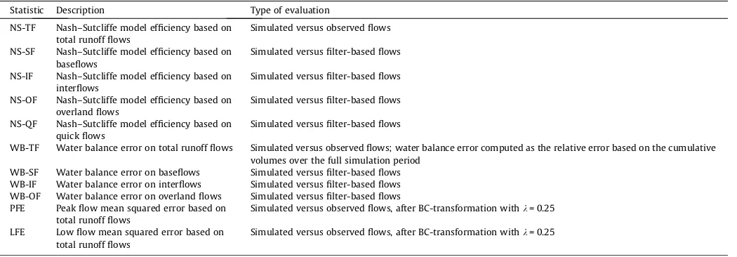
Based on these guidelines, the model goodness-of-fit statistics ofTable 1are computed in this study.
For the peak flows, next to their evaluation at the model simu-lation time step, flow – duration – frequency (QDF) resimu-lationships are also checked. The following steps are applied to derive these QDF relationships based on the observed and simulated runoff series:
– Repeat the following steps for a set of aggregation times. – The time series are aggregated using a moving average
proce-dure (length of the moving window is the aggregation time). – The aggregated series are split in independent quick flow events
and independent peak flows are extracted from the series (using the same procedure as discussed before).
– Obtain peak flows for given return periods (empirical or based on the calibrated distribution).
The following aggregation levels are considered in this study: 1, 6, 12, 24, 72, 120, 240 and 360 times the simulation time step. Given that the peak flows correspond to a partial-duration-series, the standard Generalized Pareto Distribution (GPD) is calibrated to the data. The calibration is done based on the method of weighed regression in Q–Q plots (Willems et al., 2007). After calibration of the GPDs to the data for all aggregation times, relationships are fitted between the distribution parameters and aggregation time. This is done using the method presented inTaye and Willems (2011).
2.3. Evaluation of the VHM approach
The VHM top-down approach is different from classical ap-proaches for lumped conceptual rainfall-runoff modeling in the following four main aspects:
(1) The model equations are not pre-defined, but identified in a case-specific way. Model assumptions thus are tested explic-itly based on empirical data.
(2) Model calibration is done in a step-wise way. Subsets of model parameters (related to individual model component or submodels) are identified and optimized based on subsets of additional information derived from the time series pro-cessing results.
(3) Model calibration is based on a model performance evalua-tion procedure that accounts for the influence of serial flow dependency and flow residual heteroscedasticity.
(4) Model performance evaluation explicitly involves testing the accuracy of peak and slow flow volumes as well as extreme high and low flow statistics, such that the model becomes applicable for simulation and analysis of hydrological extremes.
In order to evaluate the added value of these four features of the VHM approach, comparison is made with a number of traditional lumped conceptual modeling and model calibration methods. The four aspects above mentioned are evaluated as follows:
(1) Comparison is made with a traditional approach where modeling software with pre-defined model equations is applied. This is done for two models, NAM and PDM, which
are commonly applied in the hydrological and water engi-neering practice and literature world wide, often in combi-nation with the hydrodynamic river modeling software MIKE11 (for NAM;DHI, 2007) and InfoWorks-RS (for PDM;
Innovyze, 2011). In Flanders, these two softwares are applied as standard in support of river management and engineering. Section 2.4 gives a description of the NAM and PDM model structures and shows how these differ/com-pare with the VHM concept.
(2) Comparison is made of the VHM step-wise model calibration method with the traditional method where all model param-eters are calibrated in a single overall model optimization step by means of numerical optimization.
(3) The objective function considered for the numerical optimi-zation in (2) is changed to study the influence of the serial flow dependency and flow residual heteroscedasticity. (4) Model performance evaluation is compared after changes to
the objective function to include/exclude model goodness-fit criteria for peak and low flows and/or cumulative flow volumes.
These evaluations can be seen as a sensitivity analysis of results to the assumptions and choices made in the VHM approach.
2.4. Comparison of NAM, PDM and VHM model structures
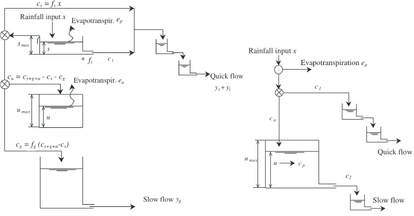
Details on the NAM model can be found inDHI (2007), Madsen (2000)andNielsen and Hansen (1973). The Probability Distributed Model (PDM) has been developed by the Centre for Ecology and Hydrology (Moore, 1985, 2007). Brief descriptions of both model structures are hereafter given. Note that we did not follow the ori-ginal descriptions and symbols used by the model developers, but that we converted these to equations and parameter symbols that are similar to the ones used for VHM. This would allow easy com-parison between the different model concepts and structures. In
Fig. 1, the NAM and PDM model structure have been converted to a representation similar to the one used for VHM.
The NAM model considers two storage reservoirs: surface stor-ages(with storage capacitysmax) and soil water storageu(capacity
umax). The surface storage reservoir is filled by rainfall input (areal catchment rainfall) and emptied by potential evapotranspirationep
and by reservoir throughflowci(contribution to interflow). When
the surface storage capacity is exceeded (s>smax) the surface reser-voir overflow volume is separated into a contributioncsto overland
flow and a contribution to infiltration. The separation between
Table 1
Statistics considered for the model performance evaluation.
Statistic Description Type of evaluation
NS-TF Nash–Sutcliffe model efficiency based on total runoff flows
Simulated versus observed flows
NS-SF Nash–Sutcliffe model efficiency based on baseflows
Simulated versus filter-based flows
NS-IF Nash–Sutcliffe model efficiency based on interflows
Simulated versus filter-based flows
NS-OF Nash–Sutcliffe model efficiency based on overland flows
Simulated versus filter-based flows
NS-QF Nash–Sutcliffe model efficiency based on quick flows
Simulated versus filter-based flows
WB-TF Water balance error on total runoff flows Simulated versus observed flows; water balance error computed as the relative error based on the cumulative volumes over the full simulation period
WB-SF Water balance error on baseflows Simulated versus filter-based flows WB-IF Water balance error on interflows Simulated versus filter-based flows WB-OF Water balance error on overland flows Simulated versus filter-based flows PFE Peak flow mean squared error based on
total runoff flows
Simulated versus observed flows, after BC-transformation withk= 0.25
LFE Low flow mean squared error based on total runoff flows
these two is time variable and depends on the overland runoff coefficientfs, which in a linear function of the relative soil
satura-tion levelu/umax:
fs¼/
u umax
ð7Þ
where
u
is the overland runoff coefficient during maximum soil saturation.NAM provides the option to consider a threshold valueutr,sfor
the soil water storage, below which the overland flow becomes zero. In that case, Eq.(7)is changed as follows:
fs¼/
uutr;s
umaxutr;s ð
8Þ
The soil storage reservoir is filled by the contributioncuto soil
storage and emptied by actual evapotranspirationea, which is a
fraction ofep, depending on the relative soil saturation level:
ea¼
u uevap
ep ð9Þ
The separation between the contribution to soil storage and the contributioncgto groundwater percolation is time variable and
de-pends on the groundwater runoff coefficientfg, which also is a
lin-ear function ofu:
fg¼
uutr;g
umaxutr;g ð
10Þ
The threshold valueutr,gis the soil water storage below which
the groundwater runoff becomes zero.
The contribution to soil storage is calculated as rest fraction:
cu¼csþgþucscg ð11Þ
The overland flowysis obtained after routing ofcsthrough two
linear reservoirs in series, with recession constantsks,1andks,2. The
inflowyiis produced by routing ofcithrough the two overland flow
routing reservoirs, whereciis the outflow from the surface storage
reservoir with recession constantkireduced by a fractionfithat
lin-early depends onu:
fi¼
uutr;i
umaxutr;i
ð12Þ
whereutr,iis the threshold value for the soil water storage below
which the interflow becomes zero.
The slow flow or baseflowygis finally obtained by routing ofcg
through a third groundwater reservoir with recession constantkg.
While VHM and NAM consider one single (lumped) soil storage reservoir, PDM considers a probability distribution to represent the spatial variability in soil storage capacity. A collection of storage reservoirs is considered (for different parts of the catchment) each with their own storage capacity. However, after assuming a spe-cific type of probability distribution, and after some recalculations of the PDM model equations, we show below that the general PDM model structure does not differ that strong from VHM and NAM.
The basic version of PDM only considers two subflows: quick and slow flows. In an initial PDM model step, actual evapotranspi-rationeais subtracted from the rainfall input. Thiseadepends (as
was the case also for VHM and NAM) on the potential evapotrans-piration ep and the soil saturation level, but using a non-linear
power equation with exponentbe:
ea¼ep 1
umaxu umax
be!
ð13Þ
Note that whenbe= 1 this evapotranspiration model becomes
equal to the one used in NAM.
From the effective rainfallx-ea, one part will contribute to quick
flow, while the other part will contribute to soil storage. Both the contributions to quick and slow flow,c1andc2, depend on the soil saturation level. The remaining rainfall fraction will contribute to soil storage, hence this last fraction will close the water balance.
The groundwater recharge depends on the soil storage by means of a power law:
c2¼
1
kgð
uutr;gumaxÞbg ð14Þ
Please note that this equation approaches a linear reservoir model for bg= 1, while it represents a non-linear reservoir for bg<>1. The parameter kg is the groundwater recharge recession
constant, and utr,g a threshold value for the soil storage below
which the groundwater recharge becomes zero. Such threshold va-lue is also considered in NAM.
After subtraction of the actual evapotranspiration and the groundwater recharge from the rainfall input, the rainfall part remaining can be calculated:
c1þu¼xeac2 ð15Þ
of which a fractionf1contributes to quick flow:
c1¼c1þuf1 ð16Þ
The relationship between this fractionf1and the soil storage
de-pends on the type of probability distribution representing the spa-tial variability in soil storage capacity cp. For the Pareto
distribution, which is frequently used (also for the study catch-ments in this paper), the following relationship is considered:
f1¼1
For that Pareto distribution, the following relationship exists betweencpand the lumped soil storage capacityumaxconsidered
in NAM and VHM:
For the quick flow routing, two linear reservoirs in series are ap-plied (recession constantskQF,1andkQF,2) together with additional time shift to the runoff results. For the slow flow routing, one linear reservoir is considered (recession constantkSF).
2.5. Calibration strategies
The NAM and PDM models are in this study calibrated using a manual calibration method that approaches the VHM calibration method as close as possible. This means that the model simulation results are optimized based on the model performance evaluation approach described in Section2.2. For the VHM model, the individ-ual submodel equations are identified and calibrated using the step-wise method outlined in Section2.1. Question raises whether an additional step where (after the initial step-wise calibration) all model parameters are fine-tuned based on overall model perfor-mance statistics would be useful (for the entire model, or for each of the different submodels). Additional question raises on the added value of the step-wise calibration and the consideration of the heteroscedasticity and temporal serial dependence properties. To answer these questions, the following parameter calibration strategies were applied to the identified VHM model structure and the model results compared:
CAL1: Step-wise manual calibration by visual inspection of model results, presented inWillems (2014)and outlined in Section2.1.
CAL2: Step-wise calibration with fine-tuning of the model parameters by numerical optimization in each step (for each sub-model). In each step (storage submodel, overland flow submodel, interflow submodel), five or six parameters are optimized. The objective function considered is the MSE of simulated versus fil-ter-based volumes of storage, overland flow or interflow (event-based and after BC-transformation withk= 0.25).
CAL3: No step-wise approach. Overall calibration of all model parameters by numerical optimization. NS-TF is considered as objective function.
CAL4: Idem CAL3 but WB-TF considered as objective function instead of NS-TF.
CAL5: Idem CAL3 but PFE considered as objective function instead of NS-TF.
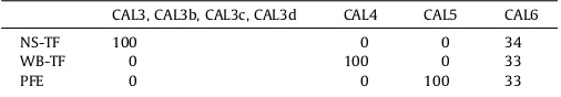
CAL6: Idem CAL3 but objective function based on NS-TF, WBE and PFE. The three statistics are as follows combined, using the weighing factors ofTable 5.
NS weight
CAL3b: Idem CAL3 but NS-TF calculated after BC-transformation withk= 0.25.
CAL3c: Idem CAL3 but NS-TF calculated based on peak flows only.
CAL3d: Idem CAL3 but NS-TF calculated based on peak flows only, and after BC-transformation with k= 0.25 (this means combining CAL3b and CAL3c).
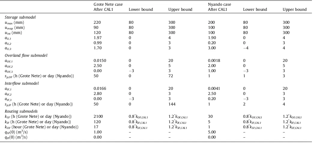
For the numerical optimization in CAL3, CAL4, CAL5 and CAL6, the Shuffled Complex Evolution Metropolis algorithm (SCEM-UA) ofVrugt et al. (2003)was applied. This algorithm consists of an adaptive and evolutionary Markov Chain Monte Carlo sampler that operates with a population of sample points divided into sub com-plexes spread out over the feasible parameter space. By means of a Bayesian method, the model parameters are treated as probabilis-tic variables having a joint posterior probability density function (pdf). This pdf captures the probabilistic beliefs about the parame-ter set in light of the observed series. The posparame-terior pdf is propor-tional to the product of a likelihood function and the prior pdf. In the algorithm, candidate points are generated using an adaptive multinormal proposal distribution, with the mean identical to the current draw in the sequence and the covariance matrix corre-sponding to the structure induced by the sample points and the complexes. The prior pdf summarizes information about the parameter set before any data is collected. This initial information consists of realistic lower and upper bounds on each of the feasible parameter space. For this study, the bounds of each parameter were identified making use of the numerical model proposal distri-bution after different calibration studies, bringing realistic bounds of parameters for each case (see Section4).
3. Study catchments
3.1. Grote Nete river catchment Belgium
The catchment of the Grote Nete river is located in the North-East of the Flanders region of Belgium. It is part of the larger Nete basin with a temperate humid climate. It has a mean July temper-ature of 16°C and a mean January temperature of 2°C. The annual rainfall depth varies from 700 to 1000 mm. The Grote Nete catch-ment has an area of 385 km2and is relatively flat. The rivers in this
catchment are typical lowland rivers with a low discharge and strong meandering. They originate from a dense network of ditches that collects seepage water. The land use in the catchment is com-posed of a mosaic of semi-natural, agricultural and urbanized areas. The soils are predominantly sandy with high hydraulic con-ductivity and intensively drained, which leads to strong interac-tions between the seasonal groundwater fluctuainterac-tions and the river discharges.
a modified Penman method, calibrated for the local conditions in Belgium (Bultot et al., 1983). Unlike rainfall data, these evaporation data can be assumed to be the same for the entire watershed. Gi-ven that snowfall rarely occurs in the region, this was not consid-ered in this study.
3.2. Nyando river catchment Kenya
The Nyando river catchment is located in the Equatorial lakes region in Western Kenya. It has a sub-humid climate with mean annual temperature of 23°C and mean annual rainfall varying from 1000 mm near Lake Victoria to over 1600 mm in the highlands. The annual rainfall pattern shows no distinct dry season. It is tri-modal with peaks during the long rains (March–May) and short rains (October–December) with the third peak in August. The rainfall is controlled by the northward and southward movement of the In-ter-Tropical Convergence Zone. The Nyando catchment has an area of about 3600 km2. Forestry and agriculture are the two
predomi-nant land use classes in the catchment. The soils are recent alluvial medium to heavy clay soils of poor drainage and structure.
The models were calibrated based on the daily river flows downstream of the catchment at Ahero bridge station. Five years of daily data (1/1/1976 – 31/12/1980) were used for calibration and the period 1/1/1986 – 31/12/1990 for validation. Model initial conditions were estimated using the same method as for the Grote Nete case. Weighted average rainfall was calculated using 38 sta-tions in and around the catchment, while four stasta-tions were used for the weighted average computation of potential
evapotranspira-tion. FAO Penman–Monteith method (Allen et al., 1998) with lim-ited data (maximum and minimum temperature) was used for estimating the potential evapotranspiration.
4. Results
4.1. Case-specific identified versus pre-defined model structure
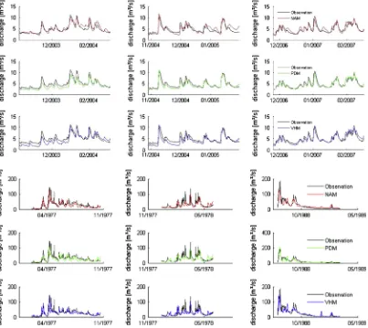
After application of the step-wise manual VHM model structure identification and calibration approach and calibration of the pre-fixed NAM and PDM model structures to the Grote Nete and Nyan-do cases, the model simulation results were evaluated based on the following model evaluation plots:
– Time series plots of total runoff flow (see Fig. 2 for three selected periods) and the subflows.
– Cumulative runoff flows (Fig. 3).
– Scatter plot of peak flows (Fig. 4) and low flows, after BC transformation.
– Empirical extreme value distribution of peak flows (Fig. 5) and low flows.
For the selection of the peak and low flows and the subflow sep-aration of the observed flow series, the parameter values ofTable 2
were considered.
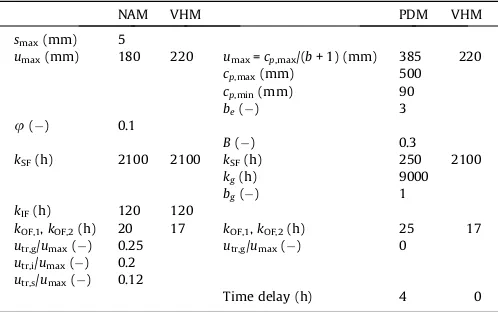
Some model parameters, e.g. the soil moisture storage capacity, have similar meaning in the different models, such that intercom-parison of their calibration values could be made. This is illustrated for the most important VHM, NAM and PDM model parameters
and the Grote Nete case inTable 3. Theumaxparameter in NAM and VHM has same meaning, and gives close values of 180 mm in NAM and 220 in VHM. This value can be directly compared with the va-lue ofcp,max/(b+ 1) in PDM, which is somewhat higher: 385 mm.
The recession constants were taken close to the empirical values obtained after the filter application, which leads to identical values forkSFin NAM and VHM. ThekSFvalue in PDM is lower but this is because the baseflow recession in PDM is also controlled by an-other parameter kg, which takes a high value after calibration.
ThekOFvalues are close in the three models, but slightly higher in PDM because no interflow is simulated in that model. The higher
kOFvalue accounts for the slower interflow recession in compari-son with the overland flow.
As can be seen inFigs. 2–5, the three models have similar per-formance in terms of total flows, peak flows and cumulative vol-umes. The NS-TF statistic has similar values for the calibration period (Table 4), but for the validation period and the Grote Nete case the PDM performance on the NS-TF index is better than for VHM (0.75 against 0.61).
Whereas the model performance is similar for the three models, further detailed investigation of the conceptual model structure highlights some systematic differences. One of these differences is shown inFig. 6, based on the relationship between the overland runoff coefficient and the relative soil moisture content. See
Willems (2014) for more details on how this relationship can be derived from the observed model input series. The VHM
Fig. 3.Cumulative runoff volumes: comparison of NAM, PDM and VHM results; Grote Nete case (left), Nyando case (right).
overland flow submodel equation is identified from the observa-tions and filter results; linear in this case. Also the NAM model con-siders a linear equation (see Section2.4), while the PDM model considers a power relation. While this leads to overestimations of the higher quick runoff coefficients (Fig. 6), this does not necessar-ily lead to a lower overall model performance. The NS-TF is even highest for the PDM model in comparison with the other two mod-els (Table 4). This means that the overestimation of the higher quick runoff coefficients is not reflected in the NS-TF or is compen-sated by biases in other components of the model.
When evaluating the models for their performance in reproduc-ing the subflow components or submodel responses, one has to be aware that the observations-based components or responses were produced by a filter or model applied to the observed series. There is obviously no guarantee that these match the actual flow compo-nents (be they observable). One could argue that when a model better represents the filter based flow components, this does not mean that it is better in absolute term, but that it better matches the hypotheses made to identify the flow components. In the case of VHM, by construction, the model is expected to be better suited to reproduce these flow components since it uses them for model structure identification. However, the filtered subflows and identi-fied subresponses provide additional information which is real, be-cause identified directly from the data, but indeed based on assumptions. The VHM model structure is based on the same assumptions, and this guarantees that the information on the main runoff subresponses obtained from the data is transferred consis-tently to the model.
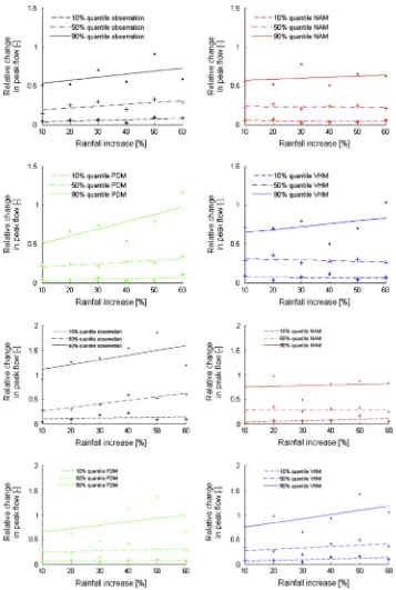
As shown before by Van Steenbergen and Willems (2012), a model with a good overall runoff performance but with biases in individual components might lead to biased impact results. Over-estimated quick runoff coefficients might, for instance, lead to overestimated impact results of climate change. This is for the PDM model of the Grote Nete case proven in Fig. 7. That figure makes intercomparison of observed versus simulated quantiles based on the cumulative frequency distributions of the quick flow changes (comparing any combination of two quick flow events se-lected from the full time series) for different classes of rainfall changes. SeeVan Steenbergen and Willems (2012)for a more de-tailed description of this method. The slopes of the 90% quantiles of relative quick flow change versus rainfall increase inFig. 7show that the PDM model of the Grote Nete overestimates the impact of rainfall changes. For the same quantiles, the NAM models of both catchments underestimate the impact of the rainfall changes. The bias is less for the VHM model. This shows the added value of testing the model for its individual components; hence of the case-specific identification of submodel structures. In both catch-ments, the observations show that the overland runoff coefficient depends in an approximate linear way on the soil saturation level (Fig. 6). When the model structure is pre-fixed, the model structure might be valid (as in the Grote Nete application is the case for NAM), but might also be biased (as for the Grote Nete is the case for PDM). When the individual submodel structures are not tested, accurate model results might still be obtained after calibration, but might lead to biased results when the model is used for extrapolation.
4.2. Comparison of calibration strategies
For VHM, the different calibration methods presented in Sec-tion2.5were applied to the Grote Nete and Nyando cases. The re-sults are compared in this section in order to investigate the added value of the step-wise manual calibration approach and the impor-tance to consider the heteroscedasticity and serial dependence of the model residuals.
Fig. 5.Empirical extreme value distribution of peak runoff flows: comparison of
NAM, PDM and VHM results; Grote Nete case (left), Nyando case (right).
Table 2
Parameters of the event and subflow separation algorithms.
Grote Nete case Nyando case
p 80 h 7 days
4.2.1. Numerical optimization settings
The numerical optimization for CAL3, CAL4, CAL5 and CAL6 by the SCEM-UA algorithm requires the number of samples, number of complexes and number of iterations to be specified. SeeVrugt et al. (2003) for more details on the definition and role of these parameters. The specification on these parameters might affect the performance of the optimization. In order to avoid that the optimization results are affected by the algorithm parameter set-tings, the sensitivity of the results after changes in the number of
complexes, number of samples and number of iterations was stud-ied. The number of iterations was found to be the most sensitive parameter together with the number of samples, whereas the number of complexes obviously depends of the number of sam-ples, taking into account that the number of samples per complex should be sufficient in order to sample with sufficient resolution the full distribution within the parameters bounds. The sensitivity analysis led to the choice of 10 for the number of complexes, 500 for the number of samples to be considered in the proposed parameter ranges, and 50,000 for the number of model iterations.
Fig. 8illustrates the sensitivity analysis; it shows that convergence is reached for the NSE optimization in the example case of CAL3c for the Grote Nete case after more 20,000 iterations and more than about 200 samples. Despite the careful selection of the prior parameter ranges (seeTable 6) and the settings of the SCEM-UA, some influence of these ranges and settings might still be present. For this reason, the results/statistics reported hereafter should not be interpreted as exact, but used for analyzing the general trends/ changes from one (set of) method(s) to the other(s). This is how the results are interpreted and summarized in this paper.
4.2.2. General evaluation
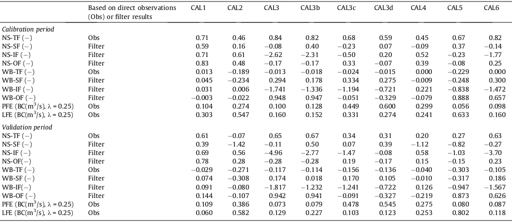
Tables 7 and 9give for both cases (Grote Nete, Belgium, and Nyando, Kenya) and for each calibration method an overview of the model parameters obtained. The corresponding goodness-of-fit statistics are for the calibration and validation periods provided inTables 8 and 10, and for the calibration period graphically visu-alized inFigs. 9–11. It is graphically clarified inFig. 10that some calibration methods show improved NS-TF statistic, but at the ex-pense of reduced model performance for the model water balance and/or subflows and/or flow extremes.
When comparing the manual, more time consuming and sub-jective method (CAL1) with the method based on step-wise numerical optimization (CAL2), the results show that both meth-ods lead to high accuracy for all the evaluation statistics. In the Grote Nete case, the manual approach leads to a highest model
Table 4
Goodness-of-fit statistics on total runoff flows: comparison of VHM, NAM and PDM results after manual calibration (CAL1); Grote Nete case (top), Nyando case (bottom) for calibration and validation periods.
Calibration period Validation period
VHM NAM PDM VHM NAM PDM
NS-TF () Obs 0.71 0.67 0.77 0.61 0.68 0.75
ME (m3/s) Obs 0.84 0.84 0.69 0.77 0.61 0.52
RMSE (m3/s) Obs 1.1 1.18 1.0 0.95 0.81 0.71
NS-QF () Filter 0.80 0.74 0.74 0.78 0.74 0.69
NS-SF () Filter 0.59 0.77 0.74 0.39 0.61 0.50
WB-TF () Obs 0.013 0.012 0.0035 0.034 0.035 0.066
PFE (BC(m3/s),k= 0.25) Obs 0.104 0.3442 0.783 0.109 0.026 0.054
LFE (BC(m3/s),k= 0.25) Obs 0.303 0.310 0.402 0.060 0.166 0.322
NS-TF () Obs 0.57 0.54 0.54 0.35 0.41 0.36
ME (m3/s) Obs 0.52 0.04 0.57 3.42 4.92 3.55
RMSE (m3/s) Obs 12.92 13.25 13.26 26.38 26.08 27.1
NS-QF () Filter 0.49 0.36 0.4 0.33 0.39 0.17
NS-SF () Filter 0.47 0.68 0.46 0.22 0.34 0.29
WB-TF () Obs 0.034 0.002 0.028 0.24 0.23 0.17
PFE (BC(m3/s),k= 0.25) Obs 0.77 0.81 0.79 0.44 0.59 0.55
LFE (BC(m3/s),k= 0.25) Obs 0.56 0.3 0.45 2.86 2.59 3.03
Table 5
Weighing factors used in the goodness-of-fit evaluation.
CAL3, CAL3b, CAL3c, CAL3d CAL4 CAL5 CAL6
NS-TF 100 0 0 34
WB-TF 0 100 0 33
PFE 0 0 100 33
Fig. 6.Evaluation of quick flow runoff coefficient versus relative soil moisture
performance for almost all statistics; while for the Nyando case CAL2 leads overall to slightly better NSE and WB results than for CAL1. The peak and low flow errors are in both cases lower for CAL1. The differences in goodness-of-fit statistics between CAL1 and CAL2 are, however, limited when compared with the other methods.
The method based on overall model optimization of NS-TF (CAL3) leads to high model performance in total flows. This meth-od obviously leads to the highest NS-TF among the methmeth-ods CAL1, CAL2 and CAL3. When results are evaluated at subflow level
(NS-SF, NS-IF, NS-OF), the step-wise approaches (CAL1 and CAL2) obviously lead to a better agreement with the filter based subflows in comparison with the methods based on numerical optimization. As discussed in Section4.1, this does not mean that these subflows will be accurate in absolute terms. However, because the subflows are extracted from the river flow observations as the main components with an order of magnitude difference in response time, they are considered indicative of the main subflow compo-nents when conceptualized. For the CAL3 results, all subflow based NS statistics even become negative. This means that the subflow
Fig. 7.Quantiles of relative change in peak flow in relation to rainfall increase: comparison of observations based changes, and NAM, PDM, VHM results; Grote Nete case
model performance is very poor; it is lower than the zero NS value obtained when the subflow would be assumed constant in time and equal to the mean filter-based subflow value.
The step-wise approach in CAL1 and CAL2 guarantees that indi-vidual submodels match the filter-based flow components. This is not the case after numerical optimization of total flow perfor-mance, as is illustrated in Figs. 12 and 13. Underestimations in one model component can indeed be compensated by overestima-tions in another component. Section 4.1explained how this can bias the impact results of scenario simulations with the model. The underestimation in OF and BF compensated by overestimation in IF (Figs. 12 and 13) leads for CAL3 to equal quality in the overall total flow performance in comparison with CAL1, but to biased im-pact results of rainfall increases. The comparison of observed ver-sus simulated cumulative frequency distributions of the overland flow changes for different classes of rainfall changes in Fig. 14
shows that the CAL3 parameter set underestimates the impact of rainfall increases. This again demonstrates the importance to
obtain accurate submodel structures, underlying an accurate over-all model performance for total flows.
Interestingly, for the Nyando case the LFE is lowest for the man-ual method. Also the PFE is among the lowest for the manman-ual meth-od; it is only lower when automatic calibration methods are applied that explicitly focus on the peak flows (CAL3c, CAL5). Also for the Grote Nete case, peak and low flow performances are good for the manual method. This is because they are explicitly taken into account by this method. The peak flow performance is also good for the methods CAL5 and CAL6 that consider this perfor-mance explicitly in the numerical optimization. When the numer-ical optimization is uniquely based on PFE (CAL5), it is trivial that lowest PFE are obtained. This is, however, at the expense of worse values for the other criteria. When the numerical optimization is done after weighing the three statistics NS-TF, WB-TF and PFE (CAL6), several model performance statistics become higher than for CAL3, CAL4 and CAL5, which are uniquely based on one statis-tic. Also the subflow related statistics in general improve for CAL6
Fig. 8.SCEM-UA convergence of the CAL3c objective function for the Grote Nete case, depending on the number of iterations and the number of samples. The number of
complexes was found to be less sensitive and was taken 10 for the results in this plot.
Table 6
Prior parameter ranges considered in the SCEM-UA optimization.
Grote Nete case Nyando case
After CAL1 Lower bound Upper bound After CAL1 Lower bound Upper bound
Storage submodel
umax(mm) 220 80 300 200 80 300
uevap(mm) 90 80 300 100 80 300
uini(mm) 120 80 300 100 80 300
aU,1 1.97 0 4 1.90 0 4
aU,2 0.99 0 3 0.20 0 3
aU,3 1.70 0 3 3.00 4 4
Overland flow submodel
aOF,1 0.0150 0 20 0.0018 0 20
aOF,2 2.50 0 5 2.00 0 5
aOF,3 0.00 3 3 1.00 3 3
sp,OF(h (Grote Nete) or day (Nyando)) 50 0 72 1 1 3
Interflow submodel
aIF,1 0.0166 0 20 0.0041 0 20
aIF,2 2.80 0 3 2.50 0 3
aIF,3 0.00 3 3 0.20 3 3
sp,IF(h (Grote Nete) or day (Nyando)) 50 0 144 1 2 4
Routing submodels
kSF(h (Grote Nete) or day (Nyando)) 2100 0.8*kOF,CAL1 1.2*kOF,CAL1 30 0.8*kOF,CAL1 1.2*kOF,CAL1
kIF(h (Grote Nete) or day (Nyando)) 120 0.8*kIF,CAL1 1.2*kIF,CAL1 5 0.8*kIF,CAL1 1.2*kIF,CAL1
kOF(hour (Grote Nete) or day (Nyando)) 17 0.8*kSF,CAL1 1.2*kSF,CAL1 1 0.8*kSF,CAL1 1.2*kSF,CAL1
qSF(0) (m3/s) 1.00 – – 5.00 – –
in comparison with CAL3. They are, however, not so good as with the step-wise methods (CAL1 and CAL2).
4.2.3. Importance to consider heteroscedasticity and serial dependence
Comparison of the statistics for CAL3 and CAL3b confirms that consideration of the heteroscedasticity in the model residual errors through the application of the BC-transformation leads to a better model performance for the low flows and slow runoff subflows. The BC-transformation avoids that more weight in given to the peak flows in comparison with the low flows, due to the higher uncertainty in the higher flow model results. For both the Grote Nete and the Nyando case, the NS-SF strongly increases, the WB-SF decreases and the LFE decreases from CAL3 to CAL3b. The same is valid but to a lesser extent for the IF related statistics. This is at the expense of a lower model performance for the peak flows: the
PFE increases from CAL3 to CAL3b in both cases. The NS-OF and WB-OF do, however, not differ much between CAL3 and CAL3b.
Consideration of the serial dependence in the calculation of the NS (see comparison of CAL3 and CAL3c) is expected to lead to a better overall performance in the peak flows. This is because less weight is given to the many strongly autocorrelated low flows in the time series. Each event gets equal weights, independent on the length of the low flow recession. The NS-OF and WB-OF strongly improve for the Grote Nete case, whereas the PFE reduces for the Nyando case. Surprisingly, the PFE increases for the Grote Nete case. This might be due to the use of the NS statistic, which opposed to CAL5 and CAL6, does not explicitly focus on the ex-treme quantiles.
When both the heteroscedasticity in the model residual errors and the serial dependence are addressed, more balanced results
Table 7
VHM parameter values after calibration; Grote Nete case.
CAL1 CAL2 CAL3 CAL3b CAL3c CAL3d CAL4 CAL5 CAL6
Storage submodel
umax(mm) 220 264 218 180 232 224 241 133 254
uevap(mm) 90 97 134 80 104 99 147 80 191
uini(mm) 120 242 109 90 116 112 121 67 127
aU,1 1.97 1.77 3.99 3.83 4.00 4.00 2.65 1.81 2.22
aU,2 0.99 1.50 1.25 1.22 1.26 1.27 1.62 1.08 0.54
aU,3 1.70 2.95 0.06 0.06 0.05 0.06 2.19 3.00 0.38
Overland flow submodel
aOF,1 0.0150 0.0282 0.0025 0.0025 0.0235 0.0225 0.0235 0.0054 0.0060
aOF,2 2.50 2.14 0.01 0.07 1.56 2.05 1.27 0.00 1.56
aOF,3 0.00 0.19 0.00 0.00 0.00 0.00 0.00 0.00 0.00
sp,OF(h) 50 59 59 50 59 59 59 59 59
Interflow submodel
aIF,1 0.0166 0.0159 0.0492 0.0386 0.0608 0.0410 0.0237 0.0220 0.0291
aIF,2 2.80 2.48 2.08 2.38 1.69 1.96 1.20 3.00 2.54
aIF,3 0.00 0.21 0.00 0.00 0.00 0.00 0.00 0.00 0.00
sp,IF(h) 50 22 22 22 22 22 22 22 22
Routing submodels
kSF(h) 2100 2100 2519 2226 1680 1680 2299 2520 2217
kIF(h) 120 120 121 100 144 144 118 104 128
kOF(h) 17 17 21 21 13 13 15 21 16
qSF(0) (m3/s) 1.00 0.90 0.90 0.90 0.90 0.90 0.90 0.90 0.90
qIF(0) (m3/s) 0.00 0.70 0.70 0.70 0.70 0.70 0.70 0.70 0.70
Table 8
Goodness-of-fit statistics for the different calibration methods; calibration and validation periods, Grote Nete case.
Based on direct observations (Obs) or filter results
CAL1 CAL2 CAL3 CAL3b CAL3c CAL3d CAL4 CAL5 CAL6
Calibration period
NS-TF () Obs 0.71 0.46 0.84 0.82 0.68 0.59 0.45 0.67 0.82
NS-SF () Filter 0.59 0.16 0.08 0.40 0.23 0.07 0.09 0.37 0.14
NS-IF () Filter 0.71 0.61 2.62 2.31 0.50 0.20 0.52 0.23 1.77
NS-OF () Filter 0.83 0.48 0.17 0.17 0.33 0.07 0.39 0.08 0.25
WB-TF () Obs 0.013 0.189 0.013 0.018 0.024 0.015 0.000 0.229 0.000
WB-SF () Filter 0.045 0.234 0.294 0.178 0.334 0.275 0.009 0.248 0.300
WB-IF () Filter 0.031 0.006 1.741 1.336 1.194 0.721 0.221 0.838 1.472
WB-OF () Filter 0.003 0.022 0.948 0.947 0.051 0.329 0.079 0.888 0.657
PFE (BC(m3/s),k= 0.25) Obs 0.104 0.274 0.100 0.128 0.449 0.600 0.299 0.056 0.098
LFE (BC(m3/s),k= 0.25) Obs 0.303 0.547 0.160 0.152 0.331 0.274 0.241 0.633 0.160
Validation period
NS-TF () Obs 0.61 0.07 0.65 0.67 0.34 0.31 0.20 0.27 0.63
NS-SF () Filter 0.39 1.42 0.11 0.50 0.07 0.39 1.12 0.82 0.27
NS-IF () Filter 0.69 0.56 4.96 2.77 1.47 0.08 0.58 1.03 3.70
NS-OF() Filter 0.78 0.28 0.28 0.28 0.19 0.17 0.15 0.15 0.23
WB-TF () Obs 0.029 0.271 0.117 0.114 0.156 0.136 0.040 0.303 0.105
WB-SF () Filter 0.074 0.308 0.174 0.018 0.170 0.105 0.010 0.317 0.186
WB-IF() Filter 0.091 0.080 1.817 1.232 1.241 0.722 0.126 0.947 1.567
WB-OF () Filter 0.144 0.107 0.942 0.941 0.091 0.327 0.219 0.873 0.626
PFE (BC(m3/s),k= 0.25) Obs 0.109 0.386 0.073 0.079 0.478 0.545 0.275 0.080 0.087
are obtained for all statistics: the NS-TF statistic decreases (from 0.838 to 0.678 for the Grote Nete, from 0.679 to 0.665 for the Nyando) but all subflows improve when CAL3d is compared with CAL3. Apart from unexpected increase in PFE for the Grote Nete case, consideration of heteroscedasticity and serial dependence in model residuals improves the automatic calibration results.
4.2.4. Improved automatic versus step-wise calibration
If we call CAL3d the improved NS-TF based automatic calibra-tion method, we can compare this improved automatic calibracalibra-tion method with the step-wise manual (CAL1) and step-wise auto-matic (CAL2) methods. We notice similar or better performance for total runoff flows for the improved automatic calibration meth-od versus the step-wise methmeth-ods, but lower performances for the NS of the subflows and for the hydrological extremes. Individual
subflow components might reach similar accuracy as the step-wise method, depending on the selected objective function, but none of the objective functions considered here allows to reach good accuracy for all (quick and slow) runoff components. The NS-IF decreased very strongly from values above 0.6 for any of the step-wise methods to negative values for most of the automatic methods. This is because only a limited fraction of the total flow is determined by this component.
4.3. Comparison of QDF-curves
In previous sections, the VHM model and approach were evalu-ated after comparison with pre-fixed model structures and other calibration strategies, but the evaluation was limited to runoff flows for the time step of the simulation and cumulative runoff volumes over the entire simulation period. Given that the
objec-Table 9
VHM parameter values after calibration; Nyando case.
CAL1 CAL2 CAL3 CAL3b CAL3c CAL3d CAL4 CAL5 CAL6
Storage submodel
umax(mm) 200 299 300 299 300 300 259 278 231
uevap(mm) 100 286 281 272 292 286 169 298 181
uini(mm) 100 103 150 150 150 150 130 139 115
aU,1 1.90 2.63 1.97 1.96 1.95 2.03 2.62 2.11 1.94
aU,2 0.20 0.61 0.20 0.18 0.19 0.24 0.79 0.43 0.15
aU,3 3.00 0.17 2.88 2.99 2.99 1.53 1.88 2.94 2.33
Overland flow submodel
aOF,1 0.0018 0.0013 0.0026 0.0025 0.0027 0.0027 0.0156 0.0048 0.0042
aOF,2 2.00 2.81 0.13 0.17 0.13 2.83 1.65 0.22 2.29
aOF,3 1.00 0.62 0.00 0.00 0.00 0.00 0.00 0.00 0.00
sp,OF(day) 1 3 1 1 1 1 1 1 1
Interflow submodel
aIF,1 0.0041 0.0028 0.0144 0.0078 0.0296 0.0123 0.0053 0.0422 0.0358
aIF,2 2.50 2.95 2.77 3.00 2.02 2.42 0.60 1.93 1.62
aIF,3 0.20 0.01 0.00 0.00 0.00 0.00 0.00 0.00 0.00
sp,IF(day) 1 2 1 1 1 1 1 1 1
Routing submodels
kSF(day) 30 30 36 36 36 36 29 31 31
kIF(day) 5 5 5 5 4 4 5 4 6
kOF(day) 1 1 2 2 2 2 1 2 1
qSF(0) (m3/s) 5.00 5.00 4.90 4.90 4.90 4.90 4.90 4.90 4.90
qIF(0)(m3/s) 0.00 0.00 0.05 0.05 0.05 0.05 0.05 0.05 0.05
Table 10
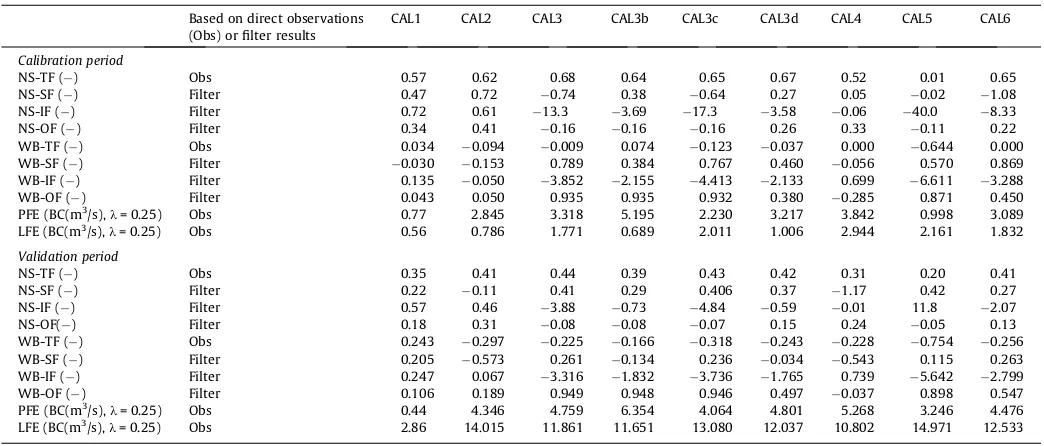
Goodness-of-fit statistics for the different calibration methods; calibration and validation periods, Nyando case.
Based on direct observations (Obs) or filter results
CAL1 CAL2 CAL3 CAL3b CAL3c CAL3d CAL4 CAL5 CAL6
Calibration period
NS-TF () Obs 0.57 0.62 0.68 0.64 0.65 0.67 0.52 0.01 0.65
NS-SF () Filter 0.47 0.72 0.74 0.38 0.64 0.27 0.05 0.02 1.08
NS-IF () Filter 0.72 0.61 13.3 3.69 17.3 3.58 0.06 40.0 8.33
NS-OF () Filter 0.34 0.41 0.16 0.16 0.16 0.26 0.33 0.11 0.22
WB-TF () Obs 0.034 0.094 0.009 0.074 0.123 0.037 0.000 0.644 0.000
WB-SF () Filter 0.030 0.153 0.789 0.384 0.767 0.460 0.056 0.570 0.869
WB-IF () Filter 0.135 0.050 3.852 2.155 4.413 2.133 0.699 6.611 3.288
WB-OF () Filter 0.043 0.050 0.935 0.935 0.932 0.380 0.285 0.871 0.450
PFE (BC(m3/s),k= 0.25) Obs 0.77 2.845 3.318 5.195 2.230 3.217 3.842 0.998 3.089
LFE (BC(m3/s),k= 0.25) Obs 0.56 0.786 1.771 0.689 2.011 1.006 2.944 2.161 1.832
Validation period
NS-TF () Obs 0.35 0.41 0.44 0.39 0.43 0.42 0.31 0.20 0.41
NS-SF () Filter 0.22 0.11 0.41 0.29 0.406 0.37 1.17 0.42 0.27
NS-IF () Filter 0.57 0.46 3.88 0.73 4.84 0.59 0.01 11.8 2.07
NS-OF() Filter 0.18 0.31 0.08 0.08 0.07 0.15 0.24 0.05 0.13
WB-TF () Obs 0.243 0.297 0.225 0.166 0.318 0.243 0.228 0.754 0.256
WB-SF () Filter 0.205 0.573 0.261 0.134 0.236 0.034 0.543 0.115 0.263
WB-IF () Filter 0.247 0.067 3.316 1.832 3.736 1.765 0.739 5.642 2.799
WB-OF () Filter 0.106 0.189 0.949 0.948 0.946 0.497 0.037 0.898 0.547
PFE (BC(m3/s),k= 0.25) Obs 0.44 4.346 4.759 6.354 4.064 4.801 5.268 3.246 4.476
tives of the paper stated that the model results are tested ‘‘for a wide range of flows and time scales’’ (see introduction section), this section evaluates the VHM model performance in the form of flow – duration – frequency (QDF) relationships.
Fig. 15shows for the Grote Nete case the empirical and cali-brated QDF-curves for the observed series versus the VHM simula-tion results after CAL1, CAL3b, CAL4, CAL5 and CAL6. The figure shows that VHM results after CAL1 match the observed flows well for the full range of time scales between 1 h and 15 days. For CAL4 systematic deviations were found for the flow extremes at small and high aggregation levels. The use of overall water balance as the only objective function indeed prevents the robust identifica-tion of parameters that control flow dynamics. QDF anomalies were also found for other automatic or non-stepwise calibration
methods, except for the methods that explicitly account for the peak flows during the calibration process (CAL5 and CAL6). No need to explain that these deviations lead to biases when the mod-el would be used for scenario investigations which involve modmod-el extrapolations.
5. Discussion and conclusion
Intercomparison between different approaches for the con-struction and calibration of lumped conceptual rainfall-runoff models was made based on two case studies. Whereas the VHM top-down approach is based on a step-wise model structure iden-tification procedure, traditional approaches for lumped conceptual rainfall-runoff modeling use a model with pre-fixed model
Fig. 9.Intercomparison of goodness-of-fit range for NS, WB and flow extremes related statistics; calibration period, Grote Nete case.
Fig. 10.Intercomparison of goodness-of-fit statistics for the different calibration methods; calibration period, Grote Nete case (darker background color for higher model
structure, e.g. NAM, PDM. This paper has shown that the identifica-tion of the model structure in a case-specific way does not lead to higher accuracy than the traditional approach when using common statistical criteria like the NS or MSE. These criteria evaluate the overall runoff performance, but it is shown that they do not
neces-sarily reflect the model performance for high and low flow ex-tremes, and submodels or subflows. AlsoGupta et al. (2009)have shown, after separation of the NS or MSE in three components rep-resenting the correlation, the bias and a measure of variability, that in order to maximize NS the total runoff variability has to be
Fig. 11.Intercomparison of goodness-of-fit range for NS, WB and flow extremes related statistics; calibration period, Nyando case.
Fig. 12.Evaluation of the rainfall fraction contributing to overland flow (left) and interflow (right) versus relative soil moisture content: comparison of CAL1 (top) and CAL3
(bottom); calibration period, Grote Nete case.
underestimated. The proposed case-specific model structure iden-tification procedure has advantages in this respect. In the Grote Nete case, a linear submodel was identified for the overland runoff coefficient based on the rainfall, PET and river flow observations. When a pre-fixed exponential submodel structure was considered, good overall model performance could be obtained after careful model calibration, but the model results become biased when extrapolated beyond the calibration range (e.g. impact simulation of climate scenarios).
Another aspect studied is the added value of the step-wise approach. When – for a fixed (prior identified) model-structure – each submodel is optimized individually, this leads to a high overall goodness-of-fit when considering all model performance aspects (total flows, subflows, peak and low flows, peak flow changes, QDF curves). One might consider the application of a global optimization step after the initial step-wise procedure. In this way, the full automatic and the manual step-wise calibration procedures can be integrated by applying the automatic calibration
0 1 2 3 4
Relative change in overland flow [-]
Cumulatieve frequency
Relative change in overland flow [-]
Cumulatieve frequency
Relative change in overland flow [-]
Cumulatieve frequency
Relative change in overland flow [-]
Cumulatieve frequency
35-45% Rainfall increase
Fig. 14.Evaluation of cumulative frequency distribution of relative change in overland flow for different classes of rainfall increase: comparison of CAL1 and CAL3 results;
calibration period, Grote Nete case.
10-1 100 101 102